GPT-3 and the actuarial landscape - An Overview of Large Language Models and Applications

Page created by Arthur Tate
 
CONTINUE READING
GPT-3 and the actuarial landscape - An Overview of Large Language Models and Applications
GPT-3 and the
actuarial landscape
An Overview of Large Language Models and Applications

CAS RPM Seminar
March 2023

A business of Marsh McLennan
GPT-3 and the actuarial landscape - An Overview of Large Language Models and Applications
CONFIDENTIALITY
Our clients’ industries are extremely competitive, and the maintenance of confidentiality with respect to our clients’ plans and data is critical.
Oliver Wyman rigorously applies internal confidentiality practices to protect the confidentiality of all client information.
Similarly, our industry is very competitive. We view our approaches and insights as proprietary and therefore look to our clients to protect our
interests in our proposals, presentations, methodologies, and analytical techniques. Under no circumstances should this material be shared with any
third party without the prior written consent of Oliver Wyman.
© Oliver Wyman
GPT-3 and the actuarial landscape - An Overview of Large Language Models and Applications
MEET THE SPEAKERS

Olivier Brown, FCAS, MAAA                           Hugo Latendresse, FCAS                           Sabrina Tan, ACAS
P&C Insurance Practice: Principal                   P&C Insurance Practice: Senior Manager           P&C Insurance Practice: Consultant
Olivier.Brown@oliverwyman.com                       Hugo.Latendresse@oliverwyman.com                 Sabrina.Tan@oliverwyman.com

Olivier Brown leads P&C Actuarial Innovation        Hugo Latendresse is a Senior Manager in Oliver   Sabrina Tan is a Consultant in Oliver Wyman’s
within Oliver Wyman’s Actuarial practice. Olivier   Wyman’s Actuarial practice. He specializes       Actuarial practice. She provides P&C actuarial
helps P&C insurers modernize their actuarial        in machine learning and automation solutions     consulting services to a variety of insurance
functions. He has worked with many insurers to      designed to improve insurance processes. Hugo    organizations. She has worked on various
improve their pricing sophistication, ratemaking,   has seven years of predictive analytics          projects in predictive analytics, process
reserving, and underwriting analytics.              experience in pricing, reserving, claims, and    improvement, pricing, and reserving.
                                                    underwriting.

© Oliver Wyman                                                                                                                                        3
GPT-3 and the actuarial landscape - An Overview of Large Language Models and Applications
OVERVIEW

                 1                     2               3
                 Intro to Natural      The Building    Actuarial Applications
                 Language Processing   Blocks of GPT

                 4                     5
                 AI: Software 2.0      Recap

© Oliver Wyman                                                                  4
GPT-3 and the actuarial landscape - An Overview of Large Language Models and Applications
1
Intro to
Natural language processing
GPT-3 and the actuarial landscape - An Overview of Large Language Models and Applications
RECENT KEY INNOVATIONS HAVE ACCELERATED ADVANCEMENTS IN NLP
Rule-based systems to simple statistical models
• First application of natural language processing (NLP)
  was for machine translation
• Initial rule-based models required significant
  manual coding                                                                        PRE-2000
• Machine learning and statistical models (N-grams,
  Markov models) and the first recurrent neural networks
  such as long short-term memory models replaced hard-                                            Use of neural networks for language modeling
  coded rules.                                                                                    • Initial uses of neural networks for next word
                                                                           2000-2017                prediction
                                                                                                  • First representations of words with dense vectors
                                                                                                    called word embeddings and algorithms capable
Attention, transformers, and large language models                                                  of learning them efficiently (Word2Vec)
• The attention mechanism along with transformer                                       2017
  architecture enable state-of-the-art performance on
  language tasks and efficient process of large datasets
• Ability to consider context in texts increased the ability                                      Generative pre-trained transformers (GPT)
  to produce human-like texts
                                                                              2018+               • OpenAI releases first version of GPT language
                                                                                                    model (2018), with GPT-2 and GPT-3 released
                                                                                                    each year thereafter
                                                                                                  • ChatGPT, fined-tuned on GPT-3.5, launched in 2022
Source: https://medium.com/nlplanet/a-brief-timeline-of-nlp-bc45b640f07d

© Oliver Wyman                                                                                                                                          6
GPT-3 and the actuarial landscape - An Overview of Large Language Models and Applications
ACCESS TO POWERFUL RESOURCES ENABLE LARGE LANGUAGE MODELS

NLP has achieved groundbreaking results through LLMs, enabled by                                                                           Compute
various modern technology                                                                                       Size of
                                                                                    Number of              training dataset             resources used
                                                                                    parameters               (Quantity of text)           for training

                 Increasing availability of text data from the internet
                                                                          BERT         110M                        16GB

                 Development of powerful computational resources          GPT          117M                        40GB
                 (GPUs and TPUs)

                                                                          RoBERTA
                                                                                       125M                       160GB
                 Frameworks for developing neural networks
                 (TensorFlow and PyTorch)
                                                                          GPT-2
                                                                                        1.5B                      800GB

                                                                                                                                             3,600+
                 Advances in ML algorithms (transformers and attention)
                                                                          GPT-3        175B                         45TB                    GPU days
                                                                                                                                           330+ MWh

© Oliver Wyman                                                                       Source: https://huggingface.co/transformers/v2.4.0/pretrained_models.html   7
GPT-3 and the actuarial landscape - An Overview of Large Language Models and Applications
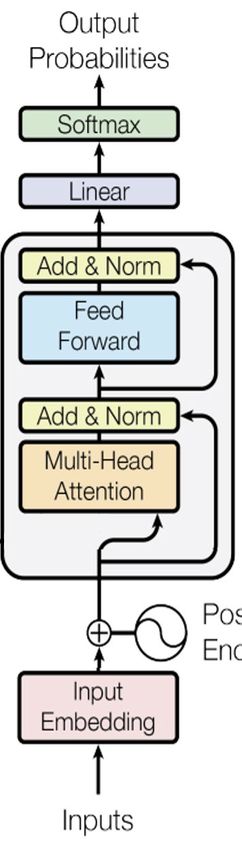
2
The building blocks of GPT
GPT-3 and the actuarial landscape - An Overview of Large Language Models and Applications
MACHINE
LEARNING 101:
GRADIENT DESCENT

© Oliver Wyman     9
GPT-3 and the actuarial landscape - An Overview of Large Language Models and Applications
MACHINE LEARNING 101: GRADIENT DESCENT

Linear Regression Model Using Formulas

Model
                  Y = β0 + β1 * X
Structure

Cost
                  Cost = Σ(predicted – actual)^2
Function

                  Slope
Formulas          β1 = (n * Σ(x*y) – Σ(x) * Σ(y)) / (n * Σ(x^2) - (Σ(x))^2)
for β
                  Intercept
coefficients
                  β0 = (Σ(y) - β1 * ΣX) / N

© Oliver Wyman                                                                10
MACHINE LEARNING 101: GRADIENT DESCENT

Linear Regression Model Using Formulas

Model
                  Y = β0 + β1 * X
Structure

Cost
                  Cost = Σ(predicted – actual)^2 = 10.7476
Function

                  Slope
Formulas          β1 = (n * Σ(x*y) – Σ(x) * Σ(y)) / (n * Σ(x^2) - (Σ(x))^2) = 10.11
for β
                  Intercept
coefficients
                  β0 = (Σ(y) - β1 * ΣX) / N = 5.15

© Oliver Wyman                                                                        11
MACHINE LEARNING 101: GRADIENT DESCENT

Linear Regression Model Using Formulas

Model
                  Y = β0 + β1 * X
Structure

Cost
                  Cost = Σ(predicted – actual)^2 = 10.7476
Function

                  Slope
Formulas          β1 = (n * Σ(x*y) – Σ(x) * Σ(y)) / (n * Σ(x^2) - (Σ(x))^2) = 10.11
for β
                  Intercept
coefficients
                  β0 = (Σ(y) - β1 * ΣX) / N = 5.15

Resulting
                  Y = 10.11 * X + 5.15
Model

© Oliver Wyman                                                                        12
MACHINE LEARNING 101: GRADIENT DESCENT

Linear Regression Model Using Formulas

Model
                  Y = β0 + β1 * X
Structure

Cost
                  Cost = Σ(predicted – actual)^2 = 10.7476
Function

                  Slope
Formulas          β1 = (n * Σ(x*y) – Σ(x) * Σ(y)) / (n * Σ(x^2) - (Σ(x))^2) = 10.11
for β
                  Intercept
                                                                                          Without those formulas,
coefficients
                  β0 = (Σ(y) - β1 * ΣX) / N = 5.15

Resulting
Model
                  Y = 10.11 * X + 5.15                                                How can we find the coefficients?

© Oliver Wyman                                                                                                            13
MACHINE LEARNING 101: GRADIENT DESCENT

Linear Regression Model Using Gradient Descent

Model
                  Y = β0 + β1 * X
Structure

Cost
                  Cost = Σ(predicted – actual)^2
Function

Formulas
for β             None!
coefficients

© Oliver Wyman                                     14
MACHINE LEARNING 101: GRADIENT DESCENT

Linear Regression Model Using Gradient Descent

Model
                  Y = β0 + β1 * X
Structure

Cost
                  Cost = Σ(predicted – actual)^2
Function

Formulas
for β             None!
coefficients

© Oliver Wyman                                     15
MACHINE LEARNING 101: GRADIENT DESCENT

Linear Regression Model Using Gradient Descent

Model
                  Y = β0 + β1 * X
Structure

Cost
                  Cost = Σ(predicted – actual)^2
Function

Formulas
for β             None!
coefficients

© Oliver Wyman                                     16
MACHINE LEARNING 101: GRADIENT DESCENT

Linear Regression Model Using Gradient Descent

Model
                                 Y = β0 + β1 * X
Structure

Cost
                                 Cost = Σ(predicted – actual)^2
Function

Formulas
for β                            None!
coefficients

Resulting                        Y = 10.11 * X + 5.15
Model
Through the two coefficients, the model “remembers” the data.

© Oliver Wyman                                                    17
REGRESSION VS CLASSIFICATION

Linear Regression                                      Multivariate Linear Regression                                  Logistic Regression

Model                                                  Model                                                           Model          Y = 1 / (1 + exp(-(β0 + β1*X 1 + β2*X 2 + …)))
                 Y = β0 + β1 * X                                      Y = β0 + β1*X 1 + β2*X 2 + β2*X 2 + β3*X 3 + …
Structure                                              Structure                                                       Structure      Y = sigmoid(β0 + β1*X 1 + β2*X 2 + …)

Cost             Sum of squared error                  Cost           Sum of squared error                             Cost           Cross-entropy
Function         Σ(predicted – actual)^2               Function       Σ(predicted – actual )^2                         Function       Σ(-(actual * log(predicted) + (1 - actual) * log(1 - predicted)))

Prediction Y can be any number                         Prediction Y can be any number                                  Prediction Y is between 0 and 1

                                                       Example: predict the sell price of a house
Example: predict the sell price of a house using one                                                                   Example: predict whether a flower is of a certain
                                                       using multiple variables (square footage, year
variable (such as square footage)                                                                                      species based on petal length and width
                                                       of construction, etc.)

© Oliver Wyman                                                                                                                                                                                      18
REGRESSION VS CLASSIFICATION

Linear Regression                                    Multivariate Linear Regression                                     Logistic Regression

Model                                                Model                                                              Model            Y = 1 / (1 + exp(-(β0 + β1*X 1 + β2*X 2 + …)))
                     Y = β0 + β1 * X                                   Y = β0 + β1*X 1 + β2*X 2 + β2*X 2 + β3*X 3 + …
Structure                                            Structure                                                          Structure        Y = sigmoid(β0 + β1*X 1 + β2*X 2 + …)

             Input                     Output              Input Layer                           Output                       Input Layer                           Output

                                                                  X1                                                                X1

                                                           Square Footage                                                      Petal Length

                                            β                                                         β                                                                 β
                 X                                                X2                                                                X2
                                         linear                                                    linear                                                            sigmoid

           Square Footage              House Price       Year of Construction                   House Price                    Petal Width                         Prob(Setosa)

                                                                  X3                                                                X3

                                                       Distance from City Center                                               Sepal Length

© Oliver Wyman                                                                                                                                                                            19
SINGLE-LABEL VS MULTI-LABEL CLASSIFICATION

Single-Label Classification                                     Multi-Label Classification Training                       Multi-Classification Training Data Example
                                                                Data Example
                                                                 Petal Length   Petal Width   Sepal Length    Species
                                                                     5.4            3.9           1.3          Setosa                     Y1 = sigmoid(β 1 0 + β 1 1* X 1 + β 1 2* X 2 + …)
Model                                                                                                                     Model
                      Y = sigmoid(β0 + β1* X 1 + β2* X 2 + …)        4.5            2.3           1.3          Setosa                     Y2 = sigmoid(β 2 0 + β 2 1* X 1 + β 2 2* X 2 + …)
Structure                                                                                                                 Structure
                                                                     4.4            3.2           1.3          Setosa                     Y3 = sigmoid(β 3 0 + β 3 1* X 1 + β 3 2* X 2 + …)
                                                                     4.8            3.0           1.4          Setosa
                                                                     5.1            3.8           1.6          Setosa
                                                                     4.6            3.2           1.4          Setosa
        Input Layer                             Output               5.3            3.7           1.5          Setosa          Input Layer                        Output Layer
                                                                     5.0            3.3           1.4          Setosa
                                                                     7.0            3.2           4.7        Versicolor
                                                                                                                                                                    β
                 X1                                                  6.4            3.2           4.5        Versicolor              X1                                      Prob(Setosa)
                                                                                                                                                                 sigmoid
                                                                     6.9            3.1           4.9        Versicolor
          Petal Length                                               5.6            2.7           4.2        Versicolor          Petal Length
                                                                     5.7            3.0           4.2        Versicolor
                                                    β                5.7            2.9           4.2        Versicolor                                             β
                 X2                                                                                                                  X2                                      Prob(versicolor)
                                                 sigmoid             6.2            2.9           4.3        Versicolor                                          sigmoid
           Petal Width                                               5.1            2.5           3.0        Versicolor
                                               Prob(Setosa)                                                                      Petal Width
                                                                     5.7            2.8           4.1        Versicolor
                                                                     6.3            2.5           5.0         Virginica
                 X3                                                  6.5            3.0           5.2         Virginica                                             β        Prob(virginica)
                                                                                                                                     X3
                                                                                                                                                                 sigmoid
                                                                     6.2            3.4           5.4         Virginica
          Sepal Length
                                                                      …              …             …              …              Sepal Length
                                                                     5.9            3.0           5.1         Virginica

© Oliver Wyman                                                                                                                                                                                20
NEURAL NETWORKS

Multi-Layer Perceptron

          Input Layer      Hidden Layer #1   Hidden Layer #2     Output Layer
                                                                                            Model        The number of nodes in the hidden layer
                                                                                            Structure    is chosen by the modeler.
                                  β                 β
                               sigmoid           sigmoid

                 X1                                               β
                                                                         Prob(Setosa)
                                                               sigmoid
                                                                                            Cost         Cross-entropy
            Petal Length          β                 β
                                                 sigmoid
                                                                                            Function     Σ(-(actual * log(predicted) + (1 - actual) * log(1 - predicted)))
                               sigmoid

                 X2                                               β
                                                               sigmoid   Prob(versicolor)

             Petal Width          β                 β                                                    All β parameters are initially set a random.
                                                 sigmoid
                                                                                            Model
                               sigmoid                                                                   The model adjusts those parameters
                                                                                            Parameters   to minimize the cost function.
                 X3                                               β      Prob(virginica)
                                                               sigmoid
            Sepal Length          β                 β
                               sigmoid           sigmoid

© Oliver Wyman                                                                                                                                                         21
BUT WHAT ABOUT
                 PREDICTING WORDS?

© Oliver Wyman                       22
NEXT WORD PREDICTION

Fundamentally, GPT-3 and ChatGPT are neural networks that constantly give a probability to what should be
the next outputted word. That’s why ChatGPT types one word at a time!

First Step: Tokenization                           Classification Problem                    Example: Tokenization of an Input

• First step of NLP any model is to convert text   • Next word prediction becomes
  into numbers, or “tokens”.                         a classification problem
• GPT-3’s tokenizer assign integers to chunks      • Input: series of tokens (a sentence)
  of characters.                                   • Output: probability distribution over
• It’s a one-to-one mapping, fixed mapping.          all tokens
  – In the input layer, “exactly” will always      • Vocab size of GPT-3 = 50,257
     be mapped to the number 3446
                                                   • The problem becomes a classification
  – In the output layer, 3446 will always            problem with 50,257 labels
     be mapped to “exactly”

                                                                                                   Source: https://platform.openai.com/tokenizer

© Oliver Wyman                                                                                                                                     23
SUMMARIZING MEANING AND REDUCING DIMENSIONALITY WITH WORD EMBEDDINGS

How to quantify meanings of words?

• Token IDs cannot be used as-is.
• Word Embedding: a large vector assigned to each token
• Values in the vector are initially assigned at random

Word Embedding Examples

 Token               Token ID       One-Hot Encoded Vector (50,000 dimensions)                              Word Embedding Vector (fewer dimensions)

 round               35634          (0, 0, 0, 0, 0, 0, …, 0, 0, 0, 0, 0, 0, 0, 0, 1, 0, …, 0, 0, 0, 0, 0)   (0.932, 0.321, 0.456, 0.571, 0.984, …, 0.654)

 ball                1894           (0, 0, 0, 0, 0, 0, …, 0, 1, 0, 0, 0, 0, 0, 0, 0, 0, …, 0, 0, 0, 0, 0)   (0.524, 0.329, 0.132, 0.134, 0.952, …, 0.213)

                                                                                                            (0.187, 0.818, 0.118, 0.901, 0.347, …, 0.221)
 net                 3262           (0, 0, 0, 0, 0, 0, …, 0, 0, 0, 0, 1, 0, 0, 0, 0, 0, …, 0, 0, 0, 0, 0)

© Oliver Wyman                                                                                                                                              24
REPRESENTING ORDER OF WORDS WITH POSITIONAL ENCODING

Network nodes need to consider multiple tokens at once. How to do that?

A naïve approach of simply taking an average or a sum of all word embedding vectors would be wrong for two reasons.
• First, obvious reason: the order of the tokens need to be considered.
Solution: Positional Encoding (see below)
• Second, less obvious reason: some words “care” more about each other than others.
Solution: Self-Attention (see next slides)

                                                                                                                   The resulting vectors represent both the
 Token           Word Embedding                                      Positional Encoding                           meaning and position of tokens.

 Name            (0.638, 0.759, 0.905, 0.243, 0.189, …, 0.900)   +   (0, 1, 0, 1, 0, ..., 0)                   =   (0.638, 1.759, 0.905, 1.243, 0.189, …, 0.900)

 the             (0.655, 0.325, 0.599, 0.91, 0.49, …, 0.726)     +   (0.031, 1.000, 0.003, 1.000, 0, ..., 0)   =   (0.686, 1.324, 0.602, 1.909, 0.490, …, 0.726)

 capital         (0.082, 0.326, 0.622, 0.418, 0.136, …, 0.344)   +   (0.062, 0.998, 0.000, 1.000, 0, ..., 0)   =   (0.144, 1.324, 0.622, 1.418, 0.136, …, 0.344)

                 (0.194, 0.294, 0.796, 0.07, 0.726, …, 0.56)
 of                                                              +   (0.094, 0.995, 0.000, 1.000, 0, ..., 0)   =   (0.288, 1.289, 0.796, 1.07, 0.726, …, 0.560)

                 (0.825, 0.943, 0.828, 0.611, 0.912, …, 0.962)
 Peru                                                            +   (0.125, 0.992, 0.000, 1.000, 0, ..., 0)   =   (0.95, 1.935, 0.828, 1.611, 0.912, …, 0.962)

© Oliver Wyman                                                                                                                                                     25
ATTENTION IS ALL YOU NEED

Self-Attention is the mechanism used by transformer models to weigh the importance of difference words in
a sentence or piece of text based on their relationships to other words.

Motivation for Self-Attention

“I can enjoy almost any music genre, but I was never enthusiastic about heavy ____.”
“I run instead of lifting, because my apartment building’s gym doesn’t have heavy ____.”

In the two sentences above:
• The words “music” and “lifting” give a lot of meaning to the token “heavy”, since those tokens help specify the context.
• The words “enthusiastic” and “apartment”, however are not very useful in finding out what is “heavy”.

Therefore, we want the next word predictions to highly depend on “music” and “lifting” and not so much on “enthusiastic” and “apartment”.

© Oliver Wyman                                                                                                                              26
CREATING KEYS, QUERIES, AND VALUES TO ALLOW SELF-ATTENTION CALCULATION

                                                                                                        Key Vectors
                                                                                                      (0.177, 0.544, …)
                                                                                                      (0.228, 0.291, …)
                                                                                                      (0.517, 0.684, …)
                                                                                                      (0.329, 0.567, …)

                                                                                                       Query Vectors
                                                       (1.909, 0.490, …)
                                                                                                      (0.258, 0.482, …)   (0.733, 0.875, …)
                             Tokenizing and Encoding   (1.418, 0.136, …)   Multiply by Query Matrix                       (0.213, 0.464, …)
“The capital of Peru ____”                                                                            (0.022, 0.887, …)
                                                       (0.288, 1.289, …)                                                  (0.533, 0.285, …)
                                                                                                      (0.618, 0.217, …)
                                                       (0.295, 1.935, …)                                                  (0.530, 0.749, …)
                                                                                                      (0.092, 0.151, …)

                                                                                                       Value Vectors
                                                                                                      (0.885, 0.857, …)
                                                                                                      (0.579, 0.423, …)
                                                                                                      (0.174, 0.136, …)
                                                                                                      (0.432, 0.932, …)

© Oliver Wyman                                                                                                                                27
COMBINING KEYS, QUERIES, AND VALUES IN SELF-ATTENTION

                                                                                             D. Unnormalized                              F. New Representation
                        A. Key                  B. Query                  C. Value               Weights          E. Normalized Weights         of “Peru”
  Preceding      Key Matrix x Previous   Query Matrix x Previous   Value Matrix x Previous
                                                                                             Key x “Peru” Query        softmax(D.)        weighted average of C.
  Tokens           Representation           Representation             Representation

  The              (0.177, 0.544, …)        (0.258, 0.482, …)         (0.885, 0.857, …)            1.798                  14%

  capital          (0.228, 0.291, …)        (0.022, 0.887, …)         (0.579, 0.423, …)            2.501                  29%
                                                                                                                                            (0.530, 0.749, …)
  of               (0.517, 0.684, …)        (0.618, 0.217, …)         (0.174, 0.136, …)            0.421                   4%

  Peru             (0.329, 0.567, …)        (0.092, 0.151, …)         (0.432, 0.932, …)            3.113                  53%

• Matrices used to obtain keys, queries, and values are common to all tokens.
• They are initialized at random and trained using gradient descent.

            Queries: vector describing what each token cares about

            Keys: vector describing what each token can inform about

            Value: vector describing information each token has to offer

© Oliver Wyman                                                                                                                                                     28
TRANSFORMER ARCHITECTURE EXAMPLE

Source: chat.openai.com/chat

© Oliver Wyman                     29
TRANSFORMER ARCHITECTURE EXAMPLE

                                                        Linear Layer                  Token ID        Value                          Token ID     Probability
                                                                                                                                                                  Sample from
                   (0.963, 0.394, …)                                                     1            0.0923                               1      0.000144
                                                                                                                   Softmax                                         distribution
                                                                                                                                                                                               Tokenizer
                                                                                         2            0.3241                               2      0.006597                          6398                     Act
                   (0.012, 0.384, …)
                                                                                         …               …                              …             …
                   (0.971, 0.410, …)
                                                                                        6398          4.9319                          6398        0.134031

                                                                                         …               …                              …             …

                                                             Value Vectors            Keys and queries weighting                                           Multi-Layer Perceptron
                  (0.574, 1.564, …)                         (0.105, 0.145, …)                     100%                 (0.105, 0.145, …)                                                          (0.963, 0.394, …)
                  (0.422, 1.555, …)                         (0.398, 0.531, …)     x              89%, 11%      =       (0.137, 0.187, …)                                                          (0.012, 0.384, …)
                  (0.983, 0.546, …)                         (0.601, 0.929, …)                 39%, 41%, 20%            (0.324, 0.460, …)                                                          (0.971, 0.410, …)

                                                                                             Self-Attention

                                                                                                                              Word Embedding                      Positional Encoding
                                                                                                    5195                      (0.574, 0.564, …)                    (0.000, 1.000, ...)            (0.574, 1.564, …)
                                                                                Tokenizer
                 Why actuaries                           Why actuaries                              43840                     (0.391, 0.555, …)             +      (0.031, 1.000, ...)     =      (0.422, 1.555, …)
                                                                                                    3166                      (0.983, 0.546, …)                    (0.062, 0.998, ...)            (0.983, 0.546, …)

                 Source: arxiv.org/pdf/1706.03762.pdf

© Oliver Wyman                                                                                                                                                                                                 30
GPT IS CAPABLE OF ZERO-SHOT LEARNING

                 Fine-tuning                       Few-shot learners       ONE-shot learners         Zero-shot learners

                                                                                                   Prompt
                                                                                                   “Can you tell me a joke
                                                                                                   about a cat and a dog?”

Update weights of pre-trained                  Model is given a few    Same as few-shot but     No demonstrations are
model by training on a dataset                 demonstrations of the   only one demonstration   allowed – the model is only
specific to the desired task                   task as conditioning,   is allowed               given a natural language
                                               but no weight updates                            description of the task
                                               are allowed

Source: https://arxiv.org/pdf/2005.14165.pdf

© Oliver Wyman                                                                                                                31
ADDING REINFORCEMENT LEARNING LAYERS AND A MODERATION API ENABLES THE
TRANSITION FROM GPT TO CHATGPT

                                                                           Fine-tune GPT-3.5

                                                                       1   ChatGPT focused language model that has been fine-tuned on
                                                                           conversational data such as short, informal sentences and specific
                                                                           conversational conventions.
         1                                                 2
                                                                           Train a reward model
                                                                       2   A labeler ranks possible responses to prompts, and this data is used
                                                                           to train a reward model to determine the final response.

                                                                           Use reinforcement learning to optimize reward
                                                                       3   An agent learns to choose the best response to a prompt by receiving
                                                                           feedback in the form of the rewards from step 2.

         4                                                 3
                                                                           Moderation endpoint

Sources:
                                                                       4   A separate language model is used to classify text as whether they violate
                                                                           content policy by being “sexual, hateful, violent, or promoting self-harm”.
https://openai.com/blog/chatgpt/
https://openai.com/blog/new-and-improved-content-moderation-tooling/

© Oliver Wyman                                                                                                                                           32
3
Actuarial applications
GPT-ENABLED TOOLS CAN HELP ACTUARIES EXECUTE THEIR WORK (1/3)
Fitting a model using GitHub Copilot

© Oliver Wyman                                                  34
GPT-ENABLED TOOLS CAN HELP ACTUARIES EXECUTE THEIR WORK (2/3)
An entire modeling process using ChatGPT and Copilot

© Oliver Wyman                                                  35
GPT-ENABLED TOOLS CAN HELP ACTUARIES EXECUTE THEIR WORK (3/3)
Using ChatGPT to debug code

© Oliver Wyman                                                  36
GPT OPENS THE DOOR TO INNOVATIVE SOLUTIONS FOR SEVERAL INSURANCE PROCESSES

  Webscraping for commercial lines underwriting            Analysis of unstructured claims data          Summarizing and searching policy contracts
    Streamline quoting process by automating            Classify/label unstructured data in claims to    Identify key provisions and search to identify
   capture of potential policyholder information      gather insights from documents such as medical              specific clauses or provisions
                                                                           reports

                  Fraud detection                                   Customer service                    Actuarial communication and report generation
  Analyze data from alternative sources to identify       Chatbots powered by GPT models can              Generate text to support actuarial analyses
   potential risks through detection of anomalies        understand natural language and provide                      and draft reports
                                                                 personalized responses

© Oliver Wyman                                                                                                                                            37
LIMITATIONS

GPT-Specific Limitations                            ChatGPT Limitations                          General Limitations of LLMs
• GPT-3 is proprietary. It would be expensive       • ChatGPT can be confidently wrong;          • LLMs are computationally expensive
  to use the API in production if thousands of        the system can write “plausible-sounding     to train and run and require vast amounts
  requests are made per day                           but incorrect or nonsensical answers”        of resources
• Insurance data often private and data can         • Can be sensitive to the phrasing           • Explainability and interpretability: can be
  be sensitive/restricted                             of the prompt                                considered a black box since these models
• Output of a general purpose LLM can rarely        • Models do not ask clarifying questions       are highly complex
  be used as-is. Additional layers have to be         when a prompt is unclear and instead       • Can perpetuate biases present in the data
  built. Classification into specific categories,     guesses the intent of the user               they are trained on, which can lead to unfair
  checks for model inaccuracy, conversion           • It is possible for the model to respond      or inaccurate predictions
  of model output (English sentences)                 to “harmful instructions or exhibit        • Requires high level of technical expertise
  into tabular data                                   biased behavior”                             to implement, maintain and use
                                                    • Supervision and adjustments are often
                                                      needed

Source: https://openai.com/blog/chatgpt

© Oliver Wyman                                                                                                                                   38
4
AI: Software 2.0
SOFTWARE IS EATING THE WORLD, AI IS EATING SOFTWARE

                                                                                                 However…
The “classical stack” of Software 1.0 is what we’re all familiar with — it is
written in languages such as Python, C++, etc. It consists of explicit                           • Applying AI to insurance and actuarial problems does not happen
instructions to the computer written by a programmer. By writing each                              automatically.
line of code, the programmer identifies a specific point in program space
with some desirable behavior. […]
                                                                                                 • There is a lot of work needed to convert our industry to Software
                                                                                                   2.0.
In contrast, Software 2.0 is written in much more abstract, human
unfriendly language, such as the weights of a neural network. […]
                                                                                                 • Who will do this work?

Software (1.0) is eating the world, and now AI (Software 2.0) is eating
software.                                                                                        • We think actuaries are ideally suited to lead this work.

                                                                ANDREJ KARPATHY
                                                                Founding Member of OpenAI
                                                                Former Director of AI at Tesla

Source: https://karpathy.medium.com/software-2-0-a64152b37c35

© Oliver Wyman                                                                                                                                                         40
WHERE TO START?
Modern software development practices are the foundation; Actuaries can learn a lot from the software world

      Design: “Simplicity is the ultimate sophistication”              Agility: Learn to “fail fast” and adapt                Testing: Foresee bugs and defects before users
   One should fall in love with the problem rather than any   It is essential to interact frequently with end users and   Automatic and timely testing of the whole code base for
   given solution. Once the problem is understood, drafts           adjust the trajectory based on their feedback.         compliance with expected behavior should be in place.
     should be presented to users before rushing to the
                      development phase.

           Version Control: Keep track of all changes                 Modularity: Reduce work duplication                     Continuous Integration: Scale the collaboration
   Allow collaborative development by tracking changes of       Maximize code understandability and reusability by        Frequent integration of all new code that compose the
      individual contributors and setting frameworks for      spreading functionalities into independent components.      application, leveraging automated testing and building
                          integration.                                                                                                        functionalities.

 Put together, these best practices ensure that code will remain easy to understand and maintain over time. It makes it easier to
 implement new functionality and integrate new technologies.
© Oliver Wyman                                                                                                                                                                      41
5
RECAP
RECAP

    We've seen exponential growth in the complexity of machine learning models, which is largely attributable to the use
    of deep learning techniques.

    Transformer models, including GPTs, have resulted in breakthrough performance on NLP tasks; the process of "self-
    attention" has been pivotal to this breakthrough.

    These breakthroughs impact all fields of work, including insurance and actuarial work.

    Converting our industry to a Software 2.0 world will require a lot of work. Actuaries are well suited to lead this work
    but need to modernize their skillset.

© Oliver Wyman                                                                                                                43
QUESTIONS
QUALIFICATIONS, ASSUMPTIONS, AND LIMITING CONDITIONS
This report is for the exclusive use of the Oliver Wyman client named herein. This report is not intended for general circulation or publication, nor is it
to be reproduced, quoted, or distributed for any purpose without the prior written permission of Oliver Wyman. There are no third-party beneficiaries
with respect to this report, and Oliver Wyman does not accept any liability to any third party.
Information furnished by others, upon which all or portions of this report are based, is believed to be reliable but has not been independently verified,
unless otherwise expressly indicated. Public information and industry and statistical data are from sources we deem to be reliable; however, we make
no representation as to the accuracy or completeness of such information. The findings contained in this report may contain predictions based on
current data and historical trends. Any such predictions are subject to inherent risks and uncertainties. Oliver Wyman accepts no responsibility for
actual results or future events.
The opinions expressed in this report are valid only for the purpose stated herein and as of the date of this report. No obligation is assumed to revise
this report to reflect changes, events, or conditions, which occur subsequent to the date hereof.
All decisions in connection with the implementation or use of advice or recommendations contained in this report are the sole responsibility of the
client. This report does not represent investment advice nor does it provide an opinion regarding the fairness of any transaction to any and all parties.
In addition, this report does not represent legal, medical, accounting, safety, or other specialized advice. For any such advice, Oliver Wyman
recommends seeking and obtaining advice from a qualified professional.
A business of Marsh McLennan
You can also read