Variability of global biome patterns as a function of initial and boundary conditions in a climate model
←
→
Page content transcription
If your browser does not render page correctly, please read the page content below
Climate Dynamics (1996) 12 : 371–379

                                                                                                 q Springer-Verlag 1996

Variability of global biome patterns as a function of initial and
boundary conditions in a climate model
Martin Claussen 1
Max-Planck-Institut für Meteorologie, Bundesstr. 55, D-20146 Hamburg, Germany

Received: 29 August 1994 / Accepted: 7 November 1995

Abstract. The use of one-way coupling of an equili-             mospheric general circulation models (AGCMs) and
brium-response vegetation, or biome, model with at-             equilibrium vegetation, or biome, models.
mospheric circulation models is critically assessed.                Due to limited computer capacity, AGCMs have
Global biome patterns from various, equally likely nu-          commonly been integrated over a few decades to yield
merical realisations of present-day climate are com-            one representation of a certain climate state. However,
pared. It has been found that the changes in global             various, albeit equally likely, numerical realisations of
biome patterns to be expected from interdecadal varia-          the same climate state generally differ (e.g. Lorenz
bility in the atmosphere affect 9–12% of the continen-          1968, 1979). As a consequence of climate variability,
tal surface (Antarctica excluded). There is no unique           biome patterns estimated from different realisations of
difference pattern, although changes are mainly in-             a climate state must differ to some degree. This varia-
duced by the variability of annual moisture availability        bility of biome patterns must not be mistaken for a re-
and, to a lesser extent, by winter temperatures. This           alistic vegetation shift, rather it reflects the uncertainty
variability of biome patterns reflects the uncertainty in       in the estimate of equilibrium vegetation patterns from
the estimate of equilibrium vegetation patterns from            finite time interval climatologies.
finite time interval climatologies. Changes in biome                The problem of (numerical) variability of biome
distributions between present-day climate and anoma-            patterns, or equilibrium climate impact patterns in gen-
ly climate, the latter induced by an increase in sea-sur-       eral, becomes important if the impact patterns of dif-
face temperatures and atmospheric CO2, are larger               ferent climate states are compared. In this case, it is
than and different in kind from the changes due to in-          necessary to estimate whether the difference between
derdecadal variability. Roughly 30% of the land sur-            impact patterns is significant. In a way, it is the same
face is affected by these changes. It appears that the          problem as differentiating between forced and free
strongest and most significant signal is seen for boreal        variations of climate (Lorenz 1979), a problem which
biomes which can be attributed to an increase in near           has not been dealt with in studies of climate impact re-
surface temperatures.                                           search (e.g. Cramer and Solomon 1993; Claussen and
                                                                Esch 1994).
                                                                    Here, the problem of the sensitivity of a biome
                                                                model to simulated climate variability is addressed by
1 Introduction                                                  analysing several, but equally likely, realisations of
                                                                present-day climate and of anomaly climate, the latter
Global vegetation patterns have been computed from              induced by enhanced sea-surface temperatures and at-
simulated climatologies (e.g. Prentice and Fung 1990;           mospheric CO2 concentrations (Sect. 3). This analysis
Henderson-Sellers 1993; Claussen and Esch 1994) and             is completed by comparing biome patterns from simu-
first attempts to incorporate continental vegetation as         lations of present-day climate and anomaly climate. In
a dynamic component of a global climate model have              particular, investigations are carried out to see whether
been undertaken (e.g. Henderson-Sellers 1993; Claus-            the change in biome patterns due to a change in cli-
sen 1994). In these studies, the vegetation structure           mate state can be identified and whether it is different
models are static equilibrium-response models. Hence,           in its kind from changes due to climate variability
there is an inconsistency at the interface between at-          (Sect. 4). The latter exercise should not be understood
                                                                as a prediction of a shift of biome patterns due to
                                                                greenhouse gas induced warming. A biome model does
1
 Present address: Potsdam Institut für Klimafolgenforschung,    not include vegetation dynamics and can, at best, pro-
Postfach 60 12 03, D-14412 Potsdam, Germany                     vide a global-scale constraint within which plant com-
372              Claussen: Variability of global biome patterns as a function of initial and boundary conditions in a climate model

munity dynamics could operate. It just serves as an ex-           Table 1. Areas (in 10 6 km 2) of biomes computed from the IIASA
ample of an analysis of different climate states. Before          climate data (Leemans and Cramer 1990) and from a 30-year si-
                                                                  mulation (T21C0 in the text) of present-day climate by using the
discussing the analyses, however, the climate model
                                                                  Hamburg climate model ECHAM at T21-resolution. (Note: polar
and the biome model used here are briefly presented               desert does not include Antarctica.)
(Sect. 2).
                                                                  Number        Biome                         IIASA       T21C0
2 Climate and biome models                                        01            Tropical rain forest           9.30        4.66
                                                                  02            Tropical seasonal forest       7.22        5.42
2.1 The climate model                                             03            Savanna                       17.40       24.19
                                                                  04            Warm mixed forest              5.44        4.76
Results of climate simulations are taken from the at-             05            Temperature decidous forest    6.24        4.39
mospheric general circulation model ECHAM devel-                  06            Cool mixed forest              7.38        5.62
oped at the Max-Planck-Institut in Hamburg. The                   07            Cool conifer forest            2.57        3.35
model physics as well as its validation are described in          08            Taiga                         13.54       13.44
detail by Roeckner et al. (1992).                                 09            Cold mixed forest              1.84        1.52
                                                                  10            Cold deciduous forest          4.49        1.33
    The climate model ECHAM (level 3) is able to si-
                                                                  11            Xerophytic woods/shrub        10.31       12.89
mulate most aspects of the observed time-mean circu-              12            Warm grass/shrub              11.20        7.41
lation and its intraseasonal variability with remarkable          13            Cool grass/shrub               6.42        4.16
skill (Roeckner et al. 1992). Nevertheless, there are a           14            Tundra                        10.12       14.89
few problems. For example, during the respective sum-             15            Hot desert                    20.04       24.24
mer seasons, there is too much precipitation over                 16            Cool desert                    4.30        0.97
                                                                  17            Polar/ice desert               2.31        6.89
South Africa and Australia and off the west coast of
Central America, whereas the rainfall over India is un-
derestimated during the summer monsoon season.
There is a lack of precipitation over the continents in           map (FAO 1974). Their predictions of global patterns
the Northern Hemisphere during summer, for example                of biomes are in good agreement with the global distri-
over the United States, over Europe, and over the dry             bution of actual ecosystem complexes being evaluated
regions of Asia. In these areas, the boundary-layer               by Olson et al. (1983). Where intensive agriculture has
temperatures are generally too high with the largest er-          obliterated the natural vegetation, comparison of pre-
ror of about 6 K.                                                 dicted biomes and observed ecosystems is, of course,
                                                                  omitted.
2.2 The biome model                                                  The global patterns of biomes computed from
                                                                  ECHAM 3 climatology agree by and large with those
In this study as well as in earlier studies (Claussen and         computed from the IIASA climate data, the north-
Esch 1994; Claussen 1994), the BIOME model of Pren-               south gradient of biome zones is particularly well rep-
tice et al. (1992) is used. In the BIOME model, 14                resented (Claussen and Esch 1994).
plant functional types are assigned climate tolerances               For a more quantitative comparison, the IIASA cli-
in terms of amplitude and seasonality of climate varia-           mate data are interpolated to the ECHAM grid and
bles. The cold tolerance of plants is expressed in terms          biomes are computed at the resolution of the climate
of minimum mean temperature of the coldest month.                 model (not shown here). It appears that ECHAM 3
Some plant types also have chilling requirements ex-              overestimates the area of savanna, though the total
pressed in terms of a maximum mean temperature of                 area of all tropical biomes is approximately correct. Li-
the coldest month. The heat requirement is a function             kewise, the total area of all deserts is fairly well esti-
of temperature sums, and the drought tolerance is re-             mated, but the extent of subtropical deserts is overesti-
lated to the annual soil moisture availability which is           mated. Details are given in Table 1. In total, the differ-
the ratio of actual and equilibrium evaporation.                  ence between biome patterns evaluated from data and
   The BIOME model predicts which plant functional                from ECHAM 3 results amounts to approximately
type can occur in a given environment, i.e. in a given            50%, i.e. 50% of the land surface on one map is occu-
set of climate variables. Competition between different           pied by different biomes on the other map. (In the fol-
plant types is treated indirectly by the application of a         lowing, “land surface” is defined as total continental
dominance hierarchy which effectively excludes certain            surface area excluding Antarctica.)
types of plants from a site, based on the presence of
others, rather than being excluded by climate (Cramer
1994). Finally, biomes are defined as combinations of             3 Comparison of biome patterns in various
dominant types.                                                   realisations of the same climate state
   Validation of the BIOME model is certainly a prob-
lem as there are very few data. Prentice et al. (1992)            3.1 Simulation of present-day climate using
have used the IIASA (International Institute of Ap-               ECHAM 3-T21
plied Systems Analysis) climate data base, described
by Leemans and Cramer (1990), and soil texture data               Biomes are compared using model results of three 10-
(to estimate soil water capacity) from the FAO soils              year integrations performed with ECHAM 3 at T21 re-
Claussen: Variability of global biome patterns as a function of initial and boundary conditions in a climate model 373
solution, i.e. the grid at which the vertical energy and forest (biome 5) in T21C1. This change occupies 0.57%
momentum exchange between the atmosphere and the of the land surface. The diagonal values yii indicate
surface are computed has a resolution of 5.67!5.67, i.e. agreement between biome maps as they list the per-
approximately 600 km!600 km at the equator. These centage of land surface occupied by the same biome on
simulations were undertaken at the Max-Planck-Insti- both maps.
tut für Meteorologie, Hamburg. Each simulation is The changes in biomes given in Table 2 can be attri-
forced by the same boundary data, in particular by the buted to differences in climate variables. It appears
same climatology of the annual cycle of SST (sea-sur- that a cool mixed forest will be replaced by a temper-
face temperatures) averaged for the years 1979 to 1988. ate deciduous forest if the winter becomes too warm so
Only the initial values differ as these runs are started that the temperature of the coldest month exceeds
from three different Januaries of the same control run. P2 7C. (For details, the reader is referred to Prentice
The three realisations are called T21C1, T21C2, et al. 1992.) On the other hand, if the annual soil mois-
T21C3. A fourth data set, T21C0, is generated by aver- ture availability is too small, less than a value of 0.75,
aging T21C1, T21C2, T21C3 to get a 30-year climatolo- then a temperate deciduous forest will rule out a cool
gy. mixed forest. Global distributions of annual moisture
The biomes computed from T21C0-3 are depicted in availability (Figs. 6, 7) and mean temperature of the
Fig. 2–5 (for allocation of colours to biomes, see Fig. coldest month (Figs. 8, 9) reveal that in Eastern Eu-
1). When comparing global biome maps estimated rope and North America, where changes from temper-
from each 10-year integration and from the 30-year av- ate deciduous forest to cool mixed forest occur (com-
erage, only approximately 6% of the land surface are pare Figs. 2–5), the annual moisture availability ex-
occupied by different biomes. When comparing biomes ceeds 0.9, but the temperature of the coldest month is
evaluated from all 10-year integrations, the difference below P2 7C. Hence, the difference between temper-
amounts to roughly 10%. ate deciduous forest and cool mixed forest can be
From where do the differences in biome maps origi- tracted to differences in winter temperatures. Follow-
nate? The largest differences are due to biome 5, i.e. ing a similar reasoning, it can be demonstrated that
temperate deciduous forest, and biome 6, cool mixed changes between cool as well as warm grass/shrub and
forest. On average, the 10-year climatologies yield less temperate deciduous forest are due to variability of an-
cool mixed forest and more temperate deciduous for- nual moisture availability and changes between warm
est than the 30-year climatology. This is the most con- mixed forest and temperate deciduous forest are due
sistent difference found when comparing all maps of to winter temperatures.
T2C1-C3 with T21C0. Difference matrices of biomes between the three
This difference can be analysed by using a “differ- 10-year integrations have also been evaluated, but are
ence matrix” given in Table 2. The matrix has to be not listed here. It turns out that these matrices have no
interpreted in the following way. A value yij in row i common structure, except that the largest changes are
and column j indicates that y% of the land surface mainly due to interdecadal variability of annual mois-
which is covered by biome i in T21C0 is covered by ture availability and, to a lesser extent, in winter tem-
biome j in T21C1. Hence, cool mixed forst (biome 6) peratures.
found in T21C0 is replaced by temperate deciduous
Table 2. Difference matrix of biome patterns from a 10-year simulation and a 30-year simulation of present-day climate, called T21C1
and T21C0 in the text, respectively
01 02 03 04 05 06 07 08 09 10 11 12 13 14 15 16 17
01 2.77 0 0 0 0 0 0 0 0 0 0 0 0 0 0 0 0
02 .26 3.58 .27 0 0 0 0 0 0 0 0 0 0 0 0 0 0
03 0 0 16.99 0 0 0 0 0 0 0 .27 0 0 0 0 0 0
04 0 0 0 2.90 0 0 0 0 0 0 .19 0 0 0 0 0 0
05 0 0 0 0 2.70 0 0 0 0 0 0 .21 0 0 0 0 0
06 0 0 0 0 .57 3.43 0 0 0 0 0 0 0 0 0 0 0
07 0 0 0 0 0 .35 1.85 .17 0 0 0 0 0 0 0 0 0
08 0 0 0 0 0 0 0 9.30 0 0 0 0 0 0 0 0 0
09 0 0 0 0 0 0 0 0 .35 0 0 0 .17 0 0 0 0
10 0 0 0 0 0 0 0 .15 0 .33 0 0 0 .28 0 0 0
11 0 0 0 .53 0 0 0 0 0 0 8.95 .26 0 0 0 0 0
12 0 0 0 0 0 0 0 0 0 0 0 4.82 .21 0 .46 0 0
13 0 0 0 0 .57 0 0 0 0 0 0 0 3.16 0 0 0 0
14 0 0 0 0 0 0 0 .15 0 0 0 0 0 10.71 0 0 0
15 0 0 0 0 0 0 0 0 0 0 0 .24 0 0 17.05 0 0
16 0 0 0 0 0 0 0 0 0 0 0 0 .24 0 0 .44 0
17 0 0 0 0 0 0 0 0 0 0 0 0 0 .10 0 0 4.81
The first row and the first column indicate the biome number (for allocation of biome numbers to biome names, see Table 1). The
meaning of matrix components yij is explained in Sect. 3.1374 Claussen: Variability of global biome patterns as a function of initial and boundary conditions in a climate model
Fig. 1. Allocation of colours used
in Figures 2–5 and 10, 11 to biomes
Fig. 2. Present biome distributions
computed from a 30-year simula-
tion, called T21C0 in the text, with
the Hamburg climate model
ECHAM 3 at T21-resolution
Fig. 3. Same as Fig. 2 but for a 10-
year integration, called T21C1
Fig. 4. Same as Fig. 3, but for a
second 10-year integration, called
T21C2
Fig. 5. Same as Fig. 4, but for a
third 10-year integration, called
T21C3Claussen: Variability of global biome patterns as a function of initial and boundary conditions in a climate model 375
Fig. 6. Global patterns of
annual moisture availability
evaluated from run T21C0
Fig. 7. Global patterns of
annual moisture availability
evaluated from run T21C1
Fig. 8. Global patterns of
mean temperature ( 7C) of
the coldest month evaluated
from run T21C0
Fig. 9. Global patterns of
mean temperature ( 7C) of
the coldest month evaluated
from run T21C1376 Claussen: Variability of global biome patterns as a function of initial and boundary conditions in a climate model
3.2 Comparison of a 10-year and a single year (1992) (called anomaly runs). As boundary conditions,
integration using ECHAM 3-T42 Perlwitz took observed climatological SST data (be-
tween 1979–1988) and superimposed the SST change
Henderson-Sellers (1993) coupled a simplified Hol- obtained from the last 10 years of a transient 100-year
dridge vegetation scheme to a climate model by feed- integration with the coupled ocean/atmosphere general
ing the information of the vegetation model to the cli- circulation model ECHAM-1-T21/LSG (Cubasch et al.
mate model at the end of each year. Hence, it should 1992). For the latter, the CO2 increase was prescribed
be worthwhile to ask how representative is a global according to the Intergovernmental Panel on Climate
distribution of biomes computed from just one year of Change (IPCC) Scenario A. In the last 10 years, the
model data. Therefore, a 10-year integration and a sin- average amount of CO2 was set to 1145 ppm and the
gle year integration using ECHAM 3 at T42 resolution global mean near-surface temperature is approximate-
(2.81257!2.81257, i.e. approximately 300 km!300 km ly 2.4 7C higher than today. As examples, biomes com-
at the equator) has been analysed using the technique puted from one of the control and one of the anomaly
outlined in the previous section. runs are shown in Figs. 10 and 11.
It was found that the difference between biome Difference matrices have been computed to investi-
maps occupies nearly a quarter (24.4%) of the land gate the differences between biome patterns between
surface. The main change is seen in savanna and tropi- the control runs and anomaly runs, respectively. Gen-
cal seasonal forest which is mainly caused by differ- erally, 9%–12% of the land surface are involved in any
ences in the annual moisture availability. The differ- change of biomes, roughly the same numbers found for
ence of 24.4% is quite strong, and is almost as large as the variability of biomes from the ECHAM 3-T21 10-
the difference between biome patterns due to a varia- year integrations. Again, no common, unique structure
tion in climate states as discussed in Sect. 4. of difference matrices is found. Changes are basically
due to the variability of annual moisture availability.
3.3 Simulation of present-day and anomaly climate
using ECHAM 3-T42
4 Comparison of biome patterns of different climate
Biomes are computed from three realisations of pres- states
ent-day climate simulations (in the following called
control runs) using 10-year integrations by ECHAM 3 In the following, the biomes computed from
at T42 resolution. The boundary conditions are inter- ECHAM 3-T42 control runs and anomaly runs are
polated from the same SST data as used for the compared. Assuming that the control runs and the
ECHAM 3-T21 simulations analysed in Sect. 3.1. anomaly runs, respectively, are statistically indepen-
Again, the boundary conditions of the three realisa- dent, nine difference matrices can be set up.
tions are identical, only the initial conditions differ in In contrast to the results of the previous section, the
the same manner as for runs T21C1-3. new difference matrices resemble each other. As an ex-
The same have been completed for three 10-year in- ample, one of the matrices is given in Table 3. All ma-
tegrations of anomaly climate performed by Perlwitz trices show a considerable change from tundra (biome
Table 3. Difference matrix of biome patterns from two 10-year simulations of present-day climate and an anomaly climate, the latter is
induced by an increase in sea-surface temperatures and atmospheric CO2 concentration
01 02 03 04 05 06 07 08 09 10 11 12 13 14 15 16 17
01 3.72 0 0 0 0 0 0 0 0 0 0 0 0 0 0 0 0
02 1.03 2.79 .58 0 0 0 0 0 0 0 0 0 0 0 0 0 0
03 0 1.24 16.21 0 0 0 0 0 0 0 .49 0 0 0 0 0 0
04 .06 .34 .67 2.27 0 0 0 0 0 0 .17 0 0 0 0 0 0
05 0 0 0 .92 1.56 .22 0 0 0 0 .20 .83 .04 0 0 0 0
06 0 0 0 0 .95 1.45 0 0 0 0 0 .52 0 0 0 0 0
07 0 0 0 0 .25 1.31 .35 .17 0 0 0 .04 .08 0 0 0 0
08 0 0 0 0 .12 .61 2.62 5.36 .08 .17 0 .04 0 0 0 0 0
09 0 0 0 0 0 0 0 0 .05 0 0 .18 .09 0 0 0 0
10 0 0 0 0 .10 .04 0 .59 .20 .48 0 0 .12 0 0 0 0
11 0 0 1.43 .20 0 0 0 0 0 0 5.51 .66 0 0 0 0 0
12 0 0 0 0 .11 0 0 0 0 0 .96 8.09 0 0 1.05 0 0
13 0 0 0 .06 0 0 0 0 0 0 .23 .83 .72 0 0 .05 0
14 0 0 0 0 0 0 0 3.58 0 .92 0 0 .05 4.43 0 .06 0
15 0 0 0 0 0 0 0 0 0 0 0 .92 0 0 16.90 0 0
16 0 0 0 0 0 0 0 0 0 0 0 .45 0 0 .34 .52 0
17 0 0 0 0 0 0 0 0 0 0 0 0 0 .59 0 0 1.89
The first row and the first column indicate the biome number (for allocation of biome numbers to biome names, see Table 1). The
meaning of matrix components yij is explained in Sect. 3.1Claussen: Variability of global biome patterns as a function of initial and boundary conditions in a climate model 377
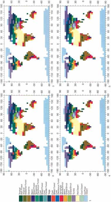
Fig. 10. Biome distributions of
present-day climate using a 10-
year integration with the Ham-
burg climate model ECHAM 3 at
T42-resolution
Fig. 11. Biome distributions of an
anomaly climate induced by an in-
crease of CO2 and sea-surface
temperatures computed using the
Hamburg climate model
ECHAM 3 at T42-resolution
14) to taiga (biome 8), with 3.5%–3.8% of the land sur- maly runs, s̄Pc̄. The last column depicts the signal-to-
face, followed by changes from taiga to cool conifer noise ratio t. According to the t-test, t is computed as:
forest (biome 7), 2.1%–3.1%, and from cool conifer
forest to cool mixed forest (biome 6), 1.3%–1.9%. All s̄Pc̄
t p ;n
differences in biomes cover approximately 30% of the ;s 2s cs 2c
land surface, i.e. the difference between biome pat-
terns due to a difference in climate states is, in this where n is the number of samples, here np3. The hy-
case, approximately three times larger than that due to pothesis s̄pc̄ can be rejected at 1% (5%) significance
interdecadal climate variability. level, if t`4.6 (2.78) or t~P4.6 (P2.78).
In Table 4, the percentage area of each biome from The difference matrix (Table 3) indicates that the
the three control runs and from the three anomaly runs change in tundra, which according to Table 4 is the
are listed in columns 2–4 and 5–7, respectively. Co- largest and most significant one, is due to a change
lumns 8 and 9 list the standard deviations sc and ss be- from tundra (in the control run) to taiga (in the ano-
tween biomes from the control runs and anomaly runs, maly run). Changes from tundra to cold mixed forest
respectively. Column 10 presents the difference be- (biome 10), to cool grass/shrub (biome 13), and to cool
tween averages of three control runs and of three ano- desert (biome 16) as well as the change from polar de-378 Claussen: Variability of global biome patterns as a function of initial and boundary conditions in a climate model
Table 4. Percentage land areas as portion of the total continental surface, Antarctica excluded, of biomes from three realisations of
present-day climate (columns 2–4) and three realisations of the anomaly climate (columns 5–7)
Percentage land area sc ss s̄Pc̄ t
01 3.70 3.71 4.15 4.58 4.81 4.73 0.25 0.12 0.86 5.30
02 4.26 4.40 4.04 4.55 4.37 6.09 0.18 0.95 0.77 1.38
03 18.34 17.86 18.05 18.95 18.81 17.67 0.24 0.70 0.39 0.91
04 3.25 3.53 3.45 3.38 3.47 3.15 0.14 0.16 P0.08 P0.65
05 3.57 3.80 3.62 3.23 3.11 3.64 0.12 0.28 P0.34 P1.94
06 2.79 2.94 2.61 3.94 3.65 3.47 0.16 0.24 0.91 5.48
07 2.02 2.06 3.15 2.98 2.98 2.72 0.14 0.22 0.83 5.56
08 8.67 9.07 8.66 9.61 9.58 10.30 0.23 0.41 1.00 3.70
09 0.20 0.33 0.37 0.45 0.35 0.39 0.09 0.05 0.09 1.54
10 1.86 1.55 1.39 1.05 1.59 1.42 0.24 0.27 P0.26 P1.24
11 7.64 7.80 7.57 7.66 7.63 7.97 0.12 0.19 0.08 0.63
12 10.07 10.21 10.53 11.56 12.61 11.55 0.24 0.61 1.63 4.34
13 1.88 1.90 1.64 1.01 1.13 1.05 0.14 0.06 P0.75 P8.33
14 9.41 9.12 9.23 5.31 5.05 5.12 0.15 0.12 P4.04 P36.83
15 18.24 17.77 18.27 18.77 18.24 17.92 0.28 0.43 0.21 0.72
16 1.50 1.39 1.58 0.70 0.64 0.69 0.09 0.03 P0.82 P14.25
17 2.51 2.48 2.48 2.03 1.90 2.03 0.02 0.08 P0.50 P10.59
For allocation of biome numbers (column 1) to biome names, see averages of present-day biomes and anomaly biomes are listed in
Table 1. Standard deviation of biomes from present-day climate column 10. The signal to noise ratio t is shown in column 11. The
simulations and from simulations of the anomaly climate are giv- hypothesis of equal averages can be rejected at a 1% significance
en in column 8 and column 9, respectively. Differences between level, if t`4.6, t~P4.6, at a 5% level, if t`2.78, t~P2.78
sert (biome 17) to tundra are only of secondary impor- 5 Conclusions
tance, although the latter change is quite significant.
By contrast, changes in savanna (biome 3) and tropical The use of one-way coupling of equilibrium-response
seasonal forest (biome 2) are as large or even larger vegetation models to AGCMs implies that there is a
than changes in cool desert (biome 16) and polar de- problem of representativeness of biome patterns. Since
sert (biome 17), but the latter are significant, the form- various, albeit equally likely, numerical representa-
er are not at all significant. The reason for this is the tions of the same climate state generally differ, the re-
great sensitivity of savanna and tropical seasonal forest sulting equilibrium vegetation patterns must also differ
to interdecadal variations in the climate model. to some degree. It has been found that for present-day
When inspecting the global distribution of climate conditions, the difference between biomes computed
parameters (not shown here), the following conclu- from three 10-year climatologies and from the corre-
sions can be drawn: the northward displacement of sponding 30-year climatology amounts to approximate-
boreal biomes, i.e. the change from polar desert to tun- ly 6% of the land surface. The difference between
dra, from tundra to taiga, and from taiga to cool mixed biome patterns derived from various 10-year integra-
forest, is associated with an increase in temperature to- tions of present-day as well as an anomaly climate var-
tals. (The annually integrated temperatures are higher ies from 9–12%. The difference between a single-year
in the anomaly climate than in the control climate.) and a 10-year integration amounts to a change in
Changes from cool grass/shrub to warm grass/shrub as biome patterns of almost 25%. There is no unique dif-
seen in the Rocky Mountains and in Manchuria (com- ference pattern, and differences in biome patterns are
pare Figs. 10, 11) can be traced back to an increase in mainly induced by changes in annual moisture availa-
summer temperatures. Differences in annual moisture bility, i.e. by the interdecadal variability of the simu-
availability are responsible for changes in central and lated hydrological cycle. The variability of the temper-
eastern Europe as well as the Congo and the Amazon- ature signal plays only a secondary rôle.
ian region. For the former, a lack of soil moisture The problem of variability of biome patterns be-
leands to a change from forests to warm grass/shrub; comes important when deciding whether biome pat-
for the latter, too much moisture converts tropical sea- terns of different climate states are in any way different
sonal forest into rain forest. or whether this difference is just due to variability. It
In conclusion, differences in biome patterns be- has been shown here that the difference between
tween the anomaly and the control runs (i.e. between biome distributions of present-day climate and an ano-
climate simulations forced by different boundary con- maly climate, the latter induced by an increase in SST
ditions) are, in this case, caused mainly by changes in and atmospheric CO2, reveals a clear and statistically
temperature in the first place. Changes in the hydro- significant signal. This signal results from an increase
logical cycle, i.e. in the annual moisture availability, of annual temperature totals as well as mean tempera-
only play a secondary rôle. tures of the coldest and warmest months. Differences
in annual moisture availability are of secondary impor-Claussen: Variability of global biome patterns as a function of initial and boundary conditions in a climate model 379
tance globally. In total, all differences affect roughly weida, both at the Max-Planck-Institut für Meteorologie, for pro-
30% of the land surface. gramming assistance. The author appreciates helpful suggestions
by Lennart Bengtsson and Martin Heimann, both at the Max-
From these results, the following conclusions con-
Planck-Institut für Meteorologie.
cerning climate and biome modeling can be drawn.
Biomes estimated from a single-years climatology are a
rather random product. Differences between biome
patterns from a single-year and a 10-year climatology References
are rather large, and almost as large as the difference
Claussen M (1994) On coupling global biome models with cli-
due to a major climate change. Henderson-Sellers
mate models. Clim Res 4 : 203–221
(1993) reports smaller interannual perentage changes Claussen M, Esch M (1994) Biomes computed from simulated cli-
of some 10%. It would be interesting to check whether matologies. Clim Dyn 9 : 235–243
this discrepancy is due to different climate variabilities Cramer W (1994) Using plant functional types in a global vegeta-
simulated by different climate models or due to the use tion model. In: Smith TM, Shugart HH, Woodward FI (eds)
of different vegetation prediction schemes. Plant functional types. Cambridge University Press, Cam-
bridge, England
It is suggested that studying the variability of biome
Cramer W, Solomon AM (1993) Climatic classification and fu-
patterns as a function of different initial conditions in ture global redistribution of agricultural land. Clim Res 3 : 97–
the climate model is a prerequisite to assessing differ- 110
ences in biome distributions between different climate Cubasch U, Hasselmann K, Höck H, Maier-Reimer E, Mikolaje-
states, a problem which has generally received little at- wicz U, Santer BD, Sausen R (1992) Time-dependent green-
tention in climate impact research. It is possible that a house warming camputations with a coupled ocean-atmos-
phere model. Clim Dyn 8 : 55–69
difference in biome patterns is large, but statistically
FAO/UNESCO (1974) Soil map of the world 1 : 5 000 000. FAO,
insignificant. For example, in this study it is found that Paris
when comparing biomes derived for present-day cli- Henderson-Sellers A (1993) Continental vegetation as a dynamic
mate and for greenhouse gas induced climate warming, component of global climate models: a preliminary assess-
changes in savanna and tropical seasonal forest are as ment. Clim Change 23 : 337–378
large or even larger than changes in hot desert and po- Leemans R, Cramer W (1991) The IIASA database for mean
monthly values of temperature, precipitation, and cloudiness
lar desert; however, the latter are quite significant, the
on a global terrestrial grid. IIASA Research Report RR-91-
former are not at all significant. The reason for this is 18, Laxenburg, Austria
the great sensitivity of savanna and tropical seasonal Lorenz EN (1968) Climatic determinism. Meteorol Monogr 8 : 1–
forest to interdecadal variations in the climate model. 3
The difference between biome patterns due to dif- Lorenz EN (1979) Forced and free variations of weather and cli-
ferent numerical representations of climate is, of mate. J Atmos Sci 36 : 1367–1376
Olson JS, Watts JA, Allison LJ (1983) Carbon in live vegetation
course, a numerical artifact. Perhaps the decay of natu-
of major world ecosystems. ORNL-5862, Oak Ridge National
ral biomes may occur rather rapidly, but the growth of Laboratory, Oak Ridge, USA
new biomes is associated with larger time scales. Cur- Perlwitz J (1992) Preliminary results of a global SST anomaly ex-
rently, there are no global models of vegetation dy- periment with a T42 GCM. Annales Geophysicae Abstracts
namics, hence we have to live with static models which of the VII General Assembly of the European Geophysical
necessitate studies like this one. In a way, the situation Society in Edinburgh, April 6–10, 1992
Prentice KC, Fung IZ (1990) The sensitivity of terrestrial carbon
of vegetation modellers resembles that of climate mod-
storage to climate change. Nature 346 : 48–51
ellers a few years ago when assessment of a green- Prentice KC, Cramer W, Harrison SP, Leemans R, Monserud
house gas induced climate change was based on non- RA, Solomon AM (1992) A global biome model based on
transient equilibrium-response simulations. plant physiology and dominance, soil properties and climate.
J Biogeogr 19 : 117–134
Acknowledgements. The authors would like to thank Colin Pren- Roeckner E, Arpe K, Bengtsson L, Brinkop S, Dümenil L, Kirk
tice, Department of Plant Ecology, Lund University, Sweden, for E, Lunkeit F, Esch M, Ponater M, Rockel B, Sausen R,
making the biome model available as well as for constructive Schlese U, Schubert S, Windelband M (1992) Simulation of
comments on an earlier version of the manuscript. Thanks are the present-day climate with the ECHAM model: impact of
also due to Jan Perlwitz, Universität Hamburg, for model data of model physics and resolution. Rep 93, Max-Planck-Institut für
the anomaly experiment, and to Monika Esch and Uwe Schulz- Meteorologie, HamburgYou can also read