LES of a laboratory-scale turbulent premixed Bunsen flame using FSD, PCM-FPI and thickened flame models
←
→
Page content transcription
If your browser does not render page correctly, please read the page content below
Available online at www.sciencedirect.com
                                                                                               Proceedings
                                                                                                     of the
                                                                                               Combustion
                                                                                                Institute
                       Proceedings of the Combustion Institute 33 (2011) 1365–1371
                                                                                       www.elsevier.com/locate/proci

LES of a laboratory-scale turbulent premixed Bunsen
flame using FSD, PCM-FPI and thickened flame models
     F.E. Hernández-Pérez *, F.T.C. Yuen, C.P.T. Groth, Ö.L. Gülder
     Institute for Aerospace Studies, University of Toronto, 4925 Dufferin Street, Toronto, ON, Canada M3H 5T6

                                          Available online 9 August 2010

Abstract

    Large-eddy simulations (LES) of a turbulent premixed Bunsen flame were carried out with three sub-
filter-scale (SFS) modelling approaches for turbulent premixed combustion. One approach is based on
the artificially thickened flame and power-law flame wrinkling models, the second approach is based on
the presumed conditional moment (PCM) with flame prolongation of intrinsic low-dimensional manifolds
(FPI) tabulated chemistry, and the third approach is based on a transport equation for the flame surface
density (FSD). A lean methane–air flame at equivalence ratio / ¼ 0:7, which was studied experimentally by
Yuen and Gülder, was considered. The predicted LES solutions were compared to the experimental data.
The resolved instantaneous three-dimensional structure of the predicted flames compares well with that of
the experiment. Flame heights and resolvable flame surface density and curvature were also examined. In
general, the average flame height was well predicted. Furthermore, the flame surface data extracted from
the simulations showed remarkably good qualitative agreement with the experimental results. The proba-
bility density functions of predicted flame curvature displayed a Gaussian-like shape centred around zero
as also observed in the experimental flame, although the experimental data showed a slightly wider profile.
The results of the comparisons highlight the weaknesses and the strengths of SFS modelling approaches
commonly used in LES of turbulent premixed flames.
Ó 2010 The Combustion Institute. Published by Elsevier Inc. All rights reserved.

Keywords: Turbulent premixed combustion; Large-eddy simulation; Thickened flame; FSD; PCM-FPI

1. Introduction                                               be resolved on LES grids and subfilter-scale (SFS)
                                                              modelling of unresolved scales is required. In this
   Large-eddy simulation (LES) is emerging as a               study, three LES SFS modelling approaches for
promising computational tool for turbulent com-               premixed turbulent combustion are compared
bustion processes [1]. However, a considerable                and applied to a turbulent Bunsen flame. One
complication for LES of turbulent premixed com-               approach is based on the artificially thickened flame
bustion is that chemical reactions occur in a thin            [2] and power-law [3] flame wrinkling models, the
reacting layer at extremely small-scales that cannot          second approach is based on the presumed condi-
                                                              tional moment (PCM) [4] with flame prolongation
                                                              of intrinsic low-dimensional manifolds (FPI) [5]
 *
   Corresponding author.                                      tabulated chemistry, and the third approach is
   E-mail address: hperez@utias.utoronto.ca                   based on a transport equation for the flame surface
(F.E. Hernández-Pérez),                                     density (FSD) [6]. Although a comparative study

1540-7489/$ - see front matter Ó 2010 The Combustion Institute. Published by Elsevier Inc. All rights reserved.
doi:10.1016/j.proci.2010.06.010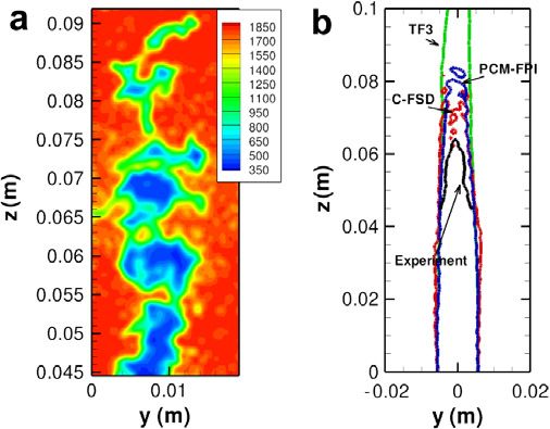
1366             F.E. Hernández-Pérez et al. / Proceedings of the Combustion Institute 33 (2011) 1365–1371

of Bunsen flames was performed recently in                                    The terms, A1 ; B1 ; B2 ; B3 , and C 1 , arise from
which LES predictions obtained using a modified                         the low-pass filtering process and require
thickened flame model were compared with exper-                         modelling. These terms are expressed as
imental data and other Reynolds-Averaged                                               @½ qð uf i uj ~ui ~uj Þ                   e
Navier–Stokes (RANS) solutions [7], there have                         A1 ¼                       @xj
                                                                                                                  ; B1 ¼  @½qð hu@xi i h~ui Þ ; B2 ¼  12
been in general few head-to-head comparative                             qð ug
                                                                       @½   j uj ui ~uj ~uj ~ui Þ                                 f e
                                                                                                      ;             C 1 ¼  @½qð Y k u@xi i Y k ~ui Þ ; B3 ¼
studies of SFS and LES modelling approaches.                                 P   @xi
                                                                                                   ð Yf        e ui Þ
                                                                                     N
                                                                           @             Dh0f;k q       k ui  Y k ~
Such studies are needed to advance LES for pre-                                     k¼1
                                                                                                                       , and must be modelled
                                                                                                 @xi
mixed combustion and clearly identify the predic-
                                                                       for closure of the filtered equation set. The subfil-
tive capabilities and limitations of SFS modelling.
                                                                       ter stresses, rij ¼                        q ð ug
                                                                                                                         i uj  ~     uj Þ, are modelled
                                                                                                                                   ui ~
A lean methane–air flame at equivalence ratio
                                                                       using an eddy-viscosity type model with
/ ¼ 0:7, which has been studied experimentally
by Yuen and Gülder [8], is considered. The capabil-                   rij ¼ 2        qmt ðSij  dij Sll =3Þ þ dij rll =3. The SFS
ities of each SFS model to predict observed behav-                     turbulent viscosity, mt , is prescribed herein by
iour are examined and compared.                                        using a one-equation model [9] for the SFS turbu-
                                                                       lent kinetic energy, ~k D . Standard gradient-based
                                                                       approximations are used in this work for the mod-
2. Favre-filtered governing equations                                   elling of the SFS fluxes B1 ; B3 , and C 1 . The subfil-
                                                                       ter turbulent diffusion term, B2 , is modelled as
    LES is based on a separation of scales, which is                   suggested by Knight et al. [10] with
achieved via a low-pass filtering procedure. Scales                      qð ug  i ui uj  ~         ui ~
                                                                                                        ui ~ uj Þ=2 ¼ rij ~   ui .
larger than the filter size, D, are resolved, whereas
scales smaller than D are modelled. Accordingly, a
relevant flow parameter, u, is filtered or Favre-fil-                     3. Thickened flame model
tered (mass-weighted filtering) to yield u     or u
                                                  ,
respectively. The Favre-filtered form of the                               One approach to modelling the turbulence/
Navier–Stokes equations governing compressible                         chemistry interaction for premixed flames is
flows of a thermally perfect reactive mixture of                        offered by the so-called thickened flame model.
gases, neglecting Dufour, Soret and radiation                          In the thickened flame model, the computed flame
effects, is used herein to describe turbulent pre-                      front structure is artificially locally thickened by a
mixed combustion processes. The equations are                          factor, F, in such a way that it can be resolved on
given by                                                               a relatively coarse LES mesh, but such that the
@ ðq
    Þ @ ðq  ~ui Þ                                                    flame speed remains unaltered [2]. An efficiency
       þ            ¼ 0;                                         ð1Þ   factor, EF , is also introduced to account for the
 @t         @xi                                                        resulting decrease in the flame Damkhöler num-
@ ðq
   ~ui Þ    @                                                       ber, Da [2]. The resulting filtered balance equation
          þ         ~ui ~uj þ dij p  sij ¼ q
                    q                           g i þ A1 ;      ð2Þ
   @t       @xj                                                        for chemical species takes the modified form
                                                                                                                      !
@ð  e
   q EÞ      @ h e                        i    @
                                                                         q Ye k Þ @ð
                                                                       @ð          q Ye k ~
                                                                                           ui Þ @              @ Ye k     EF x_ k
          þ        ðq E þ pÞ~ui þ qi            sij ~ui                     þ             ¼     EF F q
                                                                                                           Dk          þ         ;
   @t       @xi                               @xj                         @t         @xi         @xi           @xi         F
   ¼q
    gi ~ui þ B1 þ B2 þ B3 ;                                     ð3Þ
                                                                                                                                                         ð5Þ
  q Ye k Þ @ð
@ð          q Ye k ~ui Þ @ J
                             k;i
          þ              þ        ¼ x_ k þ C 1 ;                 ð4Þ   where the filtered reaction rates, x_ k , are now com-
  @t          @xi          @xi                                         puted directly by using Arrhenius law reaction
where q  is the filtered mixture density, u~i is the                   rates evaluated in terms of resolved quantities.
Favre-filtered mixture velocity, p is the filtered                         The efficiency factor, EF , is evaluated using a
mixture pressure, Ye k is the Favre-filtered mass                       power-law flame wrinkling model that assumes
                        e is the Favre-filtered total                   that the internal structure of the flame is not sig-
fraction of species k; E                                               nificantly altered by turbulence. The power-law
mixture energy (including chemical energy) given                       expression is given by [3]
            P
            N
                                                                                                     c
by     e ¼ Ye k ðhk þ Dh0 Þ  p=
       E                          q þ ug              0
                                       i ui =2; hk ; Dhf;k                                        u0
                         f;k                                                              Do
              k¼1                                                      NDo ¼ 1 þ min         ; CDo Do     ¼ EF ;          ð6Þ
and x_ k are the sensible enthalpy, heat of forma-                                        dL       sL
tion and the filtered reaction rate of species k,                       where NDo is the SFS wrinkling factor, Do is the
respectively, and gi is the acceleration due to grav-                  outer cutoff scale, and c is the power of the expres-
ity. The filtered equation of state has the form                        sion, which is taken to be 0.5 here [3]. The inner
p¼q
    R Te . The resolved stress tensor, sij , the re-                cutoff is associated with the maximum of the lam-
solved total heat flux, qi , and the resolved species                  inar flame thickness, dL , and the inverse of the
diffusive fluxes, J  k;i , are evaluated in terms of the                mean curvature of the flame, which can be esti-
filtered quantities.                                                    mated by assuming equilibrium between production
F.E. Hernández-Pérez et al. / Proceedings of the Combustion Institute 33 (2011) 1365–1371 1367
and destruction of flame surface density as 5. PCM-FPI
jhr nij ¼ D1 0
o ðuDo =sL ÞCDo , where n is a unit vec-
tor normal to the flame surface, CDo is the effi- The presumed conditional moment-FPI
ciency function proposed by Charlette et al. [3] (PCM-FPI) [4] is an approach that combines pre-
to account for the net straining of all relevant sumed probability density functions (PDF) and
scales smaller than Do and sL is the laminar flame chemistry tabulated from prototype combustion
speed. The SFS rms velocity u0Do , is calculated problems using flame prolongation of ILDM
using the expression proposed by Colin et al. [2]. (FPI) [5]. When turbulent premixed combustion
is considered, look-up tables of filtered terms
associated with chemistry are built from laminar
4. Flame surface density model premixed flamelets.
The main objective of the FPI tabulation tech-
Another approach to modelling of turbulent nique is to reduce the cost of performing reactive
premixed flames is to ignore for the most part flow computations with large chemical kinetic
the internal structure of the flame and detailed mechanisms by building databases of relevant
chemical kinetics, and represent the combustion quantities based on detailed simulations of simple
occurring at the flame front in terms of a reaction flames. Relevant chemical parameters such as spe-
progress variable. The modelled progress variable cies mass fractions or reaction rates are then
equation has the form related to a single progress of reaction variable,
Y c . For instance, any property uj (species mass
@ ðq
~cÞ @ ðq
~c~ui Þ @ q mt @~c e; fractions or reaction rates) of a steady-state lami-
þ ¼ þ qr sL q
R ð7Þ
@t @xi @xi Sct @xi nar premixed flame at equivalence ratio /0 may be
expressed as a function of position normal to the
where qr is the reactants density, R e is the Favre-fil- flame front, x, as uj ¼ uj ð/0 ; xÞ, which can then
tered flame surface area per unit mass of the mixture, be mapped to the progress variable space, Y c ,
and the product, q ~ is the flame surface area per
R, eliminating x. The resulting FPI table may then
unit volume or flame surface density (FSD). be written: uFPI j ð/0 ; Y c Þ ¼ uj ð/0 ; xÞ. Previous
The filtered quantity, R, e includes contributions studies by Fiorina et al. [12] have shown that for
from the resolved FSD and the unresolved subfil- methane–air combustion an appropriate choice
ter-scales. The latter must be modelled. A mod- for the progress of reaction is Y c ¼ Y CO2 þ Y CO .
elled transport equation for the FSD density has In the context of LES of turbulent premixed
been proposed by Hawkes and Cant [6] and is flames, a filtered quantity can be obtained via
given by Z 1
! ~j ¼
u uFPI e
j P ðc Þ dc ; ð9Þ
@ð e
q RÞ @ð e
q~ui RÞ @ q mt @ Re 0
þ
@t @xi @xi Sct @xi where c is the progress variable and Pe ðc Þ is the
pffiffiffiffiffi filtered probability density function of c, which
~ e 2
¼ CK q
Re k D bsL ð q RÞ needs to be determined. The PDF of c is taken
D 1 ~c to be a beta-distribution [13,14] and can be con-
e @~ui @ e structed from the resolved progress variable, ~c,
þ ðdij nij Þ
qR ½sL ð1 þ s~cÞM i q
R
and its SFS variance, cv ¼ cc e ~c~c. These two
@xj @xi
variables, ~c and cv , are linked to the progress of
þ sL ð1 þ s~cÞqRe @M i ; ð8Þ reaction Ye c and its SFS variance, Y cv . The filtered
@xi
progress variable is defined as the filtered progress
where M ~ ¼ rc= R e is the flamelet model for the of reaction normalized by its value at equilibrium:
surface averaged normal (c is estimated using ~c ¼ Ye c =Y Eq
c ð/0 Þ. The variance of c may be ob-
c ¼ ð1 þ sÞ~c=ð1 þ s~cÞ), a ¼ 1 M~ M,
~ and nij ¼ tained from Ye c ; Y Eq c ð/0 Þ and the variance of the
M i M j þ 1=3adij . The variable s ¼ ðT ad T r Þ=T r progress of reaction, Y cv ¼ Yg e e
c Y c Y c Y c . The
is the heat release parameter, where T ad and T r 2
are the adiabatic and the reactants temperature, expression for cv is cv ¼ Y cv =Y Eq c ð/ Þ
0 . Modelled
respectively, b is a model constant and must sat- balance equations are used to determine Y c and
isfy b P 1 for realisability requirements, a is a res- Y cv [4,13,14]. The modelled transport equation
olution factor, and CK is an efficiency function for Ye c has the form
[11]. The terms on the left hand side of the mod- " #
@ðq Ye c Þ @ð ui Ye c Þ
q~ @ Y c þ Dt Þ @ Yec
elled FSD equation represent unsteady, convec- þ ¼ ðD
q þ x_ Y c ;
tion and SFS transport effects, while the terms @t @xi @xi @xi
on the right hand side represent the production/ ð10Þ
destruction sources associated with SFS strain
and curvature, resolved strain, resolved propaga- Y c is
where x_ Y c is a source term due to chemistry, D
tion and curvature. the diffusion coefficient associated with Y c , and Dt1368 F.E. Hernández-Pérez et al. / Proceedings of the Combustion Institute 33 (2011) 1365–1371
is the turbulent diffusion coefficient used to model F ¼ 3 was utilized. Two different simulations with
SFS scalar transport. A similar balance equation the PCM-FPI model were run. In one case, species
for Y cv is used. It is important to remark that a reac- mass fractions were directly obtained from the
tion rate can be written as x_ ¼ qx_ , therefore look-up table. In the other one, the transport equa-
x_ ¼ qx~_ and Y c x_ Y ¼ q
c
Yg
cx_ Y c . The latter is a reac- tions for species were solved, reconstructing the
tion rate term appearing in the transport equation reaction rates based on a high Damköler number
for Y cv . The terms x ~_ and Yg cx_ Y c are included in approximation described in Refs. [13,14]. The chem-
Yc
the tabulated database. By introducing the segrega- istry look-up table for the PCM-FPI simulations
tion factor, S c ¼ cv =ð~cð1 ~cÞÞ, a look-up table of was generated from the steady-state solution of a
filtered quantities u ~ PCM
j ð/0 ; ~c; S c Þ, can be pre-gener- one-dimensional laminar premixed flame obtained
ated for use in subsequent LES calculations. with the Cantera package [19] for a methane–air
flame with the GRI-Mech 3.0 mechanism [20]. A
reduced number of 10 species were selected and tab-
6. Burner setup ulated based on their contributions to mixture mass
and energy [14]. The species are: CH4 ; O2 ; N2 ;
Yuen and Gülder [8] considered an axisymmet- H2 O; CO2 ; CO; H2 ; H; OH and C2 H2 . The tab-
ric Bunsen-type burner with an inner nozzle diam- ulated species mass fractions and the terms x ~_
Yc
eter of 11.2 mm to generate premixed turbulent g
and Y c x_ Y c were retrieved from the look-up table,
conical flames stabilized by annular pilot flames. which had 145 values of ~c and 25 values of S c .
Flame front images were captured using planar
The Favre-filtered transport equations described
Rayleigh scattering achieving a resolution of
above are solved on multi-block hexahedral meshes
45 lm=pixel. The Rayleigh scattering images were
employing a second-order accurate parallel finite-
converted into temperature field and further pro-
volume scheme [21]. The inviscid flux at each cell
cessed to provide the temperature gradient and
face is evaluated using limited linear reconstruc-
two-dimensional curvature. Particle image veloci-
tion [22] and Riemann-solver based flux functions
metry was used to measure the instantaneous
[23,24], while the viscous flux is evaluated utilizing
velocity field for the experimental conditions.
a hybrid average gradient-diamond path method
The flame considered in this work corresponds
[25]. A explicit second-order Runge–Kutta scheme
to a lean premixed methane–air flame at an equiv-
was used to time-march the solutions. Parallel
alence ratio of / ¼ 0:7 and atmospheric pressure.
implementation of the finite-volume scheme has
The turbulence at the burner exit was character-
been carried out via domain decomposition using
ized by a non-dimensional turbulence intensity
the C++ programming language and the MPI
u0 =sL ¼ 14:38 and an integral length scale
(message passing interface) library.
Lt ¼ 1:79 mm. The mixture of reactants was at a
temperature of 300 K and its mean velocity was
15.6 m/s. The flame lies in the thickened wrinkled
flame or thin reaction zone of the turbulent pre- 7. Results and discussion
mixed combustion diagram and the corresponding
turbulent Reynolds number is 324. In what follows, the numerical solutions
In the simulations, a cylindrical domain having obtained with the different models are identified
a diameter of 0.05 m and a height of 0.1 m was as PCM-FPI, PCM-FPI-RR, TF3 and C-FSD
employed and discretized with a grid consisting results. The difference between the PCM-FPI
of 1,638,400 hexahedral cells. The pilot flame and PCM-FPI-RR is that the species mass frac-
was approximated by a uniform inflow of hot tions were transported and their reaction rates
combustion products at a velocity of 16.81 m/s. were reconstructed for PCM-FPI-RR, whereas
For the burner exit, a uniform mean inflow of species mass fraction were directly read from the
reactants with superimposed turbulent fluctua- look-up table for PCM-FPI.
tions was prescribed. The velocity fluctuations
were pre-generated using the procedure developed 7.1. Instantaneous flame front
by Rogallo [15] and superimposed onto the mean
inflow velocity using Taylor’s hypothesis of frozen Three-dimensional views of the predicted
turbulence. The same velocity fluctuations were instantaneous flame surface, identified by the iso-
used for all the simulations. therm Te ¼ 1076 K, are displayed in Fig. 1 corre-
For the numerical results presented herein, ther- sponding to time t ¼ 4 ms after the initiation of
modynamic and molecular transport properties of the simulation, for which a quasi-steady flame
each mixture component are prescribed using the structure has been achieved in each case. The sim-
database compiled by Gordon and McBride ulated flames exhibit a highly wrinkled surface
[16,17]. In the thickened flame simulation, meth- and the scale of wrinkling becomes larger near
ane–air chemistry was represented by a one-step the tips of the flames. Moreover, the overall pre-
reaction mechanism as described by Westbrook dicted flame structure is quite similar for each of
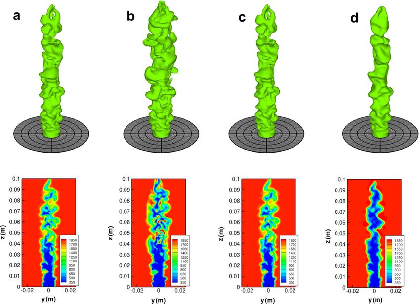
and Dryer [18] and a constant thickening factor the SFS models, although the FSD model resultsF.E. Hernández-Pérez et al. / Proceedings of the Combustion Institute 33 (2011) 1365–1371 1369
Fig. 1. Instantaneous flame iso-surface Te ¼ 1076 K at 4 ms after the initiation of the simulations. (a) PCM-FPI, (b) C-
FSD, (c) PCM-FPI-RR, (d) TF3.
can be attributed to the fact that turbulent struc-
tures smaller than the flame front thickness are
unable to wrinkle the thickened flame front.
More details of the internal structure of the
flames can be seen in the lower part of Fig. 1,
where planar cuts of the four instantaneous solu-
tions are shown. The solutions are in close agree-
ment with each other up to nearly 3 cm above the
bottom line. Further downstream, particularly in
the region above 5 cm of the burner exit, clear dif-
ferences are noticeable. Pockets of unburned reac-
tants can be identified in Fig. 1a–c, which are not
present in Fig. 1d. For direct comparison, a fil-
tered instantaneous image of the experimental
flame is shown in Fig. 2a obtained with a filter-
Fig. 2. Instantaneous filtered temperature from the width equal to that of the computations. As it
experiment and 0.5 contour of the averaged cT map can be seen, the numerical simulations are able
from the experiment and the simulations. (a) Filtered to reproduce, at least qualitatively, key features
image, (b) hcT i ¼ 0:5. of the experimental flame front.
7.2. Flame surface density
would seem to exhibit the most wrinkling and the
thickened flame shows considerably less resolved To extract the flame surface density from the
wrinkling than its counterparts. experimental data, the Rayleigh scattering images
In the C-FSD case of Fig. 1b, a more spread were processed to obtain progress variable fields
flame is observed. The PCM-FPI (Fig. 1a) and based on temperature. This progress variable is
PCM-FPI-RR (Fig. 1c) solutions display a nearly defined as cT ¼ ðT T u Þ=ðT b T u Þ, where T is
identical structure, whereas the artificially thick- the local temperature, T u is the unburnt gas tem-
ened flame (Fig. 1d) is considerably less wrinkled perature and T b is the fully burnt gas temperature.
than those of the other models. This observation The two-dimensional (2D) maps of the FSD were1370 F.E. Hernández-Pérez et al. / Proceedings of the Combustion Institute 33 (2011) 1365–1371
0.6 1.8
Experiment
1.6 Filtered Exp.
Flame surface density (1/mm)
0.5 PCM-FPI
1.4 PCM-FPI-RR
Normalized frequency
TF3
0.4 1.2 C-FSD
1
0.3
0.8
0.2 Experiment 0.6
FilteredExp.
PCM-FPI 0.4
0.1 PCM-FPI-RR
TF3 0.2
C-FSD
0 0
0 0.2 0.4 0.6 0.8 1 -5 0 5
cT 2D curvature (1/mm)
Fig. 3. 2D flame surface density extracted from the Fig. 4. PDF of 2D curvature corresponding to a
experimental data and LES simulations. progress variable cT ¼ 0:5.
computed by using the method developed by ulations show very good qualitative agreement
Shepherd [26], in which instantaneous flame front with the experimental FSD profiles.
edges are superimposed onto the averaged cT map
to calculate the length over area ratio for a given 7.3. Flame front curvature
cT . The same procedure was then applied to 2D
slices of the resolved temperature field obtained Two-dimensional curvature was also extracted
from the LES simulations. Since LES provides from instantaneous experimental images and slices
solutions of filtered variables, it is more appropri- of the numerical solutions. The curvature PDFs of
ate to compare the numerical results with filtered the experimental data, filtered experimental data
experimental data. The experimental temperature and the different LES solutions, corresponding to
images were therefore first filtered with a top-hat cT ¼ 0:5 are shown in Fig. 4. The PDFs display a
filter having a characteristic size of two times the Gaussian-type shape centred around zero. It can
average cell size of the LES computational grid. be highlighted that filtering the experimental data
The total number of post-processed experimental leads to a narrower PDF, which is due to the fact
images was 300 and, for each LES simulation, that filtering removes small-scale wrinkled struc-
the 2D slices were extracted from 19 instanta- tures having larger curvatures. All the LES solu-
neous snapshots of the numerical solution sepa- tions exhibit a narrow PDF as compared to the
rated by 0.25 ms. experimental ones. It can also be seen that the PDFs
Predictions of the average map of cT ¼ 0:5 for obtained from the C-FSD, PCM-FPI and PCM-
the three SFS models are compared with the map FPI-RR simulations nearly overlap with each
obtained from the Rayleigh scattering images in other and the filtered experimental results, whereas
Fig. 2b. Although it is quite evident that the thick- the PDF obtained from the TF3 simulation is the
ened flame model over-predicts the average flame most narrow. These trends indicate that more small-
height by a considerable margin, both C-FSD and scale wrinkling is captured by the C-FSD and
PCM-FPI models yield flame heights (7 cm and PCM-FPI models, as compared to the thickened
7.75 cm, respectively) that agree very well with flame model.
the experimental value, which is estimated to be
about 6.5 cm based on the cT ¼ 0:5 contour.
The 2D FSD values extracted from the simula- 8. Concluding remarks
tions and the experiment are compared in Fig. 3.
It can be seen that all the FSD profiles obtained The present comparison of SFS model results
from the simulations qualitatively reproduce the for LES of a turbulent lean premixed methane–air
trends observed in the experimental data. In all Bunsen flame to the experimental results of Yuen
the profiles the maximum FSD value is found and Gülder [8] has revealed a number of deficiencies
around cT ¼ 0:5. The peak FSD values obtained in the thickened flame model, even with a relatively
from the simulations are higher than the experi- small value of 3 for the thickening factor. The flame
mental ones. Despite quantitative discrepancies height was significantly over-predicted, the instan-
observed, 2D FSD profiles obtained from the sim- taneous flame front exhibits noticeably less wrinklingF.E. Hernández-Pérez et al. / Proceedings of the Combustion Institute 33 (2011) 1365–1371 1371
than the actual experimental flame, and the References
resolved curvature of the flame front is under-pre-
dicted. These deficiencies would be even more pro- [1] H. Pitsch, Annu. Rev. Fluid Mech. 38 (2006) 453–482.
nounced if a large thickening factor were adopted [2] O. Colin, F. Ducros, D. Veynante, T. Poinsot,
as is more typically used. Phys. Fluids 12 (2000) 1843–1863.
In contrast, the performance of the C-FSD, [3] F. Charlette, C. Meneveau, D. Veynante, Combust.
PCM-FPI, and PCM-FPI-RR models was found Flame 131 (2002) 159–180.
[4] P. Domingo, L. Vervisch, S. Payet, R. Hauguel,
to be much better, with all three approaches provid- Combust. Flame 143 (2005) 566–586.
ing predictions that agree both qualitatively and [5] O. Gicquel, N. Darabiha, D. Thévenin, Proc.
quantitatively with key aspects of the flame observed Combust. Inst. 28 (2000) 1901–1908.
in the experiment. The resolved flame structure and [6] E.R. Hawkes, R.S. Cant, Combust. Flame 126
wrinkling, average flame height, and resolved flame (2001) 1617–1629.
surface and curvature all compare well with experi- [7] A. De, S. Acharya, Combust. Sci. Tech. 181 (2009)
ment. The FSD model appears to be best suited 1231–1272.
for describing the evolution and dynamics of the [8] F.T.C. Yuen, O.L. Gülder, Proc. Combust. Inst. 32
flame surface, yielding slightly better predictions of (2009) 1747–1754.
[9] A. Yoshizawa, K. Horiuti, J. Phys. Soc. Jpn. 54
these quantities, but is lacking in terms its connec- (1985) 2834–2839.
tion of flame area to reaction rates. The PCM-FPI [10] D. Knight, G. Zhou, N. Okong’o, V. Shukla, Paper
model seems more rubust and can be applied more 98-0535, AIAA, January 1998.
widely to premixed, non-premixed, and partially [11] C. Meneveau, T. Poinsot, Combust. Flame 86 (1991)
premixed flames, although at the expense of higher 311–332.
computational costs (computational costs of the [12] B. Fiorina, O. Gicquel, L. Vervisch, S. Carpentier,
LES with the PCM-FPI-RR SFS model were about N. Darabiha, Proc. Combust. Inst. 30 (2005) 867–874.
55% more than those of the C-FSD model). Future [13] P. Domingo, L. Vervisch, D. Veynante, Combust.
research will involve further comparisons of the SFS Flame 152 (2008) 415–432.
[14] J. Galpin, A. Naudin, L. Vervisch, C. Angelberger,
models for the premixed flame considered here at O. Colin, P. Domingo, Combust. Flame 155 (2008)
other turbulence intensities and to compare predic- 247–266.
tions of turbulent burning rate to experimental esti- [15] R.S. Rogallo, NASA Tech. Memo. 81315 (1981).
mates of those values. [16] S. Gordon, B.J. McBride, NASA Ref. Pub. 1311
(1994).
[17] B.J. McBride, S. Gordon, NASA Ref. Pub. 1311
Acknowledgements (1996).
[18] C.K. Westbrook, F.L. Dryer, Combust. Sci. Tech.
27 (1981) 31–43.
Computational resources for performing all of [19] D. Goodwin, H.K. Moffat, Cantera, available at
the calculations reported herein were provided by .
the SciNet High Performance Computing Consor- [20] G.P. Smith, D.M. Golden, M. Frenklach, N.W.
tium at the University of Toronto and Compute/ Moriarty, B. Eiteneer, M. Goldenberg et al., GRI-
Calcul Canada through funding from the Canada Mech 3.0, available at .
ince of Ontario, Canada. The first author grate- [21] X. Gao, C.P.T. Groth, J. Comput. Phys. 229 (2010)
fully acknowledges the support received from the 3250–3275.
[22] T.J. Barth, Paper 93-0668, AIAA, January 1993.
Mexican National Council for Science and Tech- [23] P.L. Roe, J. Comput. Phys. 43 (1981) 357–372.
nology (CONACYT) and the European Commu- [24] M.-S. Liou, J. Comput. Phys. 214 (2006) 137–170.
nity’s Sixth Framework Programme (Marie Curie [25] S.R. Mathur, J.Y. Murthy, Numer. Heat Transfer
Early Stage Research Training Fellowship) under 31 (1997) 191–215.
contract number MEST-CT-2005-020426. [26] I. Shepherd, Proc. Combust. Inst. 26 (1996) 373–379.You can also read