The stress shadow problem in physics-based aftershock forecasting: Does incorporation of secondary stress changes help?
←
→
Page content transcription
If your browser does not render page correctly, please read the page content below
The stress shadow problem in physics-based aftershock
     forecasting: Does incorporation of secondary stress
                        changes help?
                                       M. Segou, T. Parsons

     To cite this version:
    M. Segou, T. Parsons. The stress shadow problem in physics-based aftershock forecasting: Does
    incorporation of secondary stress changes help?. Geophysical Research Letters, American Geophysical
    Union, 2014, 41 (11), pp.3810-3817. �10.1002/2013GL058744�. �hal-02196089�

                                 HAL Id: hal-02196089
                https://hal.archives-ouvertes.fr/hal-02196089
                                    Submitted on 16 Sep 2021

    HAL is a multi-disciplinary open access            L’archive ouverte pluridisciplinaire HAL, est
archive for the deposit and dissemination of sci- destinée au dépôt et à la diffusion de documents
entific research documents, whether they are pub- scientifiques de niveau recherche, publiés ou non,
lished or not. The documents may come from émanant des établissements d’enseignement et de
teaching and research institutions in France or recherche français ou étrangers, des laboratoires
abroad, or from public or private research centers. publics ou privés.
                                              Copyright
PUBLICATIONS
Geophysical Research Letters
RESEARCH LETTER The stress shadow problem in physics-based
10.1002/2013GL058744
aftershock forecasting: Does incorporation
Key Point:
• Only few aftershocks inside stress
of secondary stress changes help?
shadows can be linked to M. Segou1,2 and T. Parsons1
secondary effects
1
United States Geological Survey, Menlo Park, California, USA, 2Now at GeoAzur/CNRS, Valbonne, France
Supporting Information:
• Readme
• Figure S1 Abstract Main shocks are calculated to cast stress shadows across broad areas where aftershocks occur.
• Figure S2 Thus, a key problem with stress-based operational forecasts is that they can badly underestimate aftershock
• Appendixes S1 and S2
occurrence in the shadows. We examine the performance of two physics-based earthquake forecast models
• Table S1
• Table S2 (Coulomb rate/state (CRS)) based on Coulomb stress changes and a rate-and-state friction law for their
predictive power on the 1989 Mw = 6.9 Loma Prieta aftershock sequence. The CRS-1 model considers the
Correspondence to: stress perturbations associated with the main shock rupture only, whereas CRS-2 uses an updated stress field
M. Segou,
with stresses imparted by M ≥ 3.5 aftershocks. Including secondary triggering effects slightly improves
segou@geoazur.unice.fr
predictability, but physics-based models still underestimate aftershock rates in locations of initial negative
stress changes. Furthermore, CRS-2 does not explain aftershock occurrence where secondary stress changes
Citation:
enhance the initial stress shadow. Predicting earthquake occurrence in calculated stress shadow zones
Segou, M., and T. Parsons (2014), The stress
shadow problem in physics-based after- remains a challenge for stress-based forecasts, and additional triggering mechanisms must be invoked.
shock forecasting: Does incorporation of
secondary stress changes help?, Geophys.
Res. Lett., 41, 3810–3817, doi:10.1002/
2013GL058744. 1. Introduction
Received 2 APR 2014
Operational aftershock forecasting is usually based either on statistics derived from our empirical knowledge of
Accepted 19 MAY 2014 the system [Ogata, 1998] or on physical models that anticipate seismicity by invoking rate-and-state friction laws
Accepted article online 21 MAY 2014 combined with static stress change calculations [e.g., Stein, 1999; Toda et al., 2005]. Researchers have not reached
Published online 6 JUN 2014
consensus on static stress change effects, suggesting, for example, that there is a strong spatial correlation
between stress shadows and seismicity rate reduction [Toda et al., 2012], a total absence of stress shadows [Felzer
and Brodsky, 2005], or alteration of primary focal mechanisms [Mallman and Parsons, 2008]. Usually correlation
between static stress increases and major historic earthquakes [Stein, 1999] and/or aftershocks considers just the
main shock perturbation and long-term aftershock occurrence [e.g., Toda and Stein, 2003]. In the near-source
region it is difficult to identify aftershocks triggered by static or dynamic stress changes because both are
expected to increase seismicity rates [Freed, 2005; Hill and Prejean, 2007]. Felzer and Brodsky [2005] find distinct
distance decay related to dynamically triggered aftershocks from earthquake sources with M2-6 [Richards-Dinger
et al., 2010]. More recently, Parsons et al. [2012] found that microseismicity patterns within aftershock sequences
cannot be fully explained by main shock static stress changes, since they are partly caused from secondary
triggering. Marsan [2005] suggested that, at large scale, an aftershock distribution is constrained by the early
stress release and clustering inside stress increased regions, which does not evolve much through the sequence.
In this study we investigate whether continuous updating of the stress field by perturbations caused from
smaller magnitude aftershocks (M ≥ 3.5) improves the predictive power of forecast models based on a rate/
state friction law and static stress changes. We compare the predictive power of two Coulomb rate/state
(CRS) forecast models, the CRS-1 model, which considers the stress perturbations associated with the main
shock rupture only, and the CRS-2 model, which corresponds to a time evolving stress field incorporating
stresses imparted by aftershocks within three clusters near the epicentral region of 1989 Loma Prieta Mw 6.9
in Northern California. We then compare the number of forecasted events with M ≥ 1.6 from both
implementations with observations. Finally, we discuss how our results contribute in the development of
future operational forecasting efforts and understanding earthquake triggering processes.
2. Data and Methods
There are two main characteristics that make the Loma Prieta aftershock sequence a compelling case study
for secondary triggering studies: (1) aftershock clusters that initiated within the first 24–30 h after the main
SEGOU AND PARSONS ©2014. American Geophysical Union. All Rights Reserved. 3810Geophysical Research Letters 10.1002/2013GL058744
Figure 1
SEGOU AND PARSONS ©2014. American Geophysical Union. All Rights Reserved. 3811Geophysical Research Letters 10.1002/2013GL058744
shock and that persisted for about 2 years, and (2) the absence of aftershocks on parts of the Loma Prieta
rupture plane that slipped during the main shock, as seen in other California main shocks [Mendoza and
Hartzell, 1988]. We select three aftershock clusters (labeled A, B, and C in Figure 1, panel A) that occurred in
calculated stress shadows for studying secondary triggering effects.
In our Coulomb/rate-state (CRS) model framework, the seismicity rate R is a function of a state variable γ that
evolves in time under a shear-stressing rate according to the Dieterich [1994] equations (see Appendix S1 in
the supporting information). We include effects from nine M ≥ 5.0 Northern California ruptures that occurred
between 1980 and 1989 into the state variable (γn 1) calculation (see Table S1). Aftershock locations are
taken from the high precision relocated catalog of Waldhauser and Schaff [2008], with uncertainties in the
horizontal and vertical direction of approximately 1 km and 2 km, respectively.
The main components of the CRS model implementation are (1) 3-D static stress change calculations with
target depth sampled every 0.4 km, (2) rate-state constitutive parameters, stressing rate i, and the term Aσ
(where A is a constant, and σ is a normal stress), and (3) a reference seismicity rate (M ≥ 1.6) from the period
1974–1980 (Advanced National Seismic Network (ANSS) catalog). We assume uniform reference rates
because there is limited information and sparse seismicity in the epicentral area of Loma Prieta main shock
before 1980. However, we note that the selection of the background seismicity model is important in physics-
based forecasting as in Northern California [Segou et al., 2013] and in other locations [Hainzl et al., 2010]. We
calculate the mean Coulomb stress change using all available main shock source models at 3-D points for
varying coefficients of friction (0.2 ≤ μ ≤ 0.8) and the 95% confidence interval. We note that stressing rate τ
and the Aσ term are related through τ̇ ¼ Aσ=ta [Dieterich, 1994], where ta is the aftershock duration. In this
implementation we choose to fix the stressing rate for the San Andreas Fault Peninsula segment based on
Parsons [2002] and vary the term Aσ from 0.2 to 2 bars with a 0.2 bar sampling interval. Although previous
studies for California suggest a good fit for Aσ = 0.5 [Toda et al., 2005; Segou et al., 2013], we use 10 different
values here to assess sensitivity of this parameter on forecast aftershock rates [e.g., Hainzl et al., 2010].
We use five Loma Prieta source models [Lisowski et al., 1990; Beroza, 1991; Marshall et al., 1991; Steidl et al., 1991;
Wald, 1991] for calculating main shock static stress changes (Figure 1, panel A) because our aftershock clusters
lie within ~10 km of the rupture plane, and calculations at these locations might be sensitive to small
differences in the source slip distributions [Simpson and Reasenberg, 1994; Steacy et al., 2004]. We calculate
stress changes on specific planes, based on pre–main shock predominant geology features [McLaughlin et al.,
1972; Clark, 1981; Aydin and Page, 1984; Segou et al., 2013], at varying target depths with spatial resolution in
both vertical and horizontal direction 2 km. The predominant geology grid receiver planes are represented
by (1) vertical dextral strike slip (strike: N40°W, rake: 180°) for target depths less than 10 km, corresponding to
the Santa Cruz Mountains section of the San Andreas Fault, (2) dextral reverse oblique planes (rake 135°)
trending N57°W dipping 60°SW that represent the Zayante-Vergeles fault zone, and that mark the merge of the
thrust component of the Santa Cruz Mountains section of the San Andreas Fault zone for target depths greater
than 10 km. The above interpretation is for the central part of the Loma Prieta rupture, and is based on the
Loma Prieta aftershock interpretation of Dietz and Ellsworth [1990, 1997]. They find that although there is a
diversity of focal mechanisms within the aftershock sequence [see also Beroza and Zoback, 1993; Kilb et al.,
1997], strike slip faulting dominates the upper 10 km, whereas dextral reverse faulting similar to the main shock
mechanism occurs between 10 and 18 km.
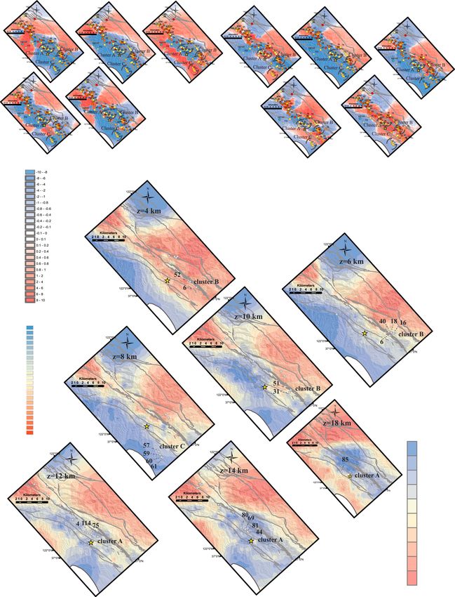
Figure 1. Panel (A) Coulomb stress changes following Loma Prieta Mw = 6.9 main shock resolved for target depths (A–E)
z = 14 and (a–e) z = 6 km using the source models of (A-a) Beroza [1991], (B-b) Lisowski et al. [1990], (C-c) Marshall et al.
[1991], (D-d) Wald 1991, and (E-e) Steidl et al. [1991] for friction coefficient μ = 0.4. Aftershocks are taken from the relocated
catalog of Waldhauser and Schaff [2008]; early aftershocks (first day) corresponding to warm colors going to colder ones for
longer time intervals (>1 year). The (A–C) aftershock clusters under analysis are identified. Both CRS models are based on a
3-D static stress change calculation sampling target depth interval 2 km taking into consideration varying friction
coefficients (0.2 ≤ μ ≤ 0.8). Panel (B) Map view of the probability that a location is under stress decrease (PDCFFGeophysical Research Letters 10.1002/2013GL058744
We assess parameter sensitivity in Coulomb stress modeling by varying friction coefficients (0.2 ≤ μ ≤ 0.8) for
each main shock model at each target depth. However, there would be too little time immediately after a
main shock to develop complex source models, so a uniform slip model like that of Lisowski et al. [1990] (see
Figure 1, panel A, b), perhaps with stochastic variations, would be more realistic on operational time scales.
For each target depth we map the Spatial Cumulative Density Function (SpatialCDF) that answers the
question, What is the probability that a specific location is subject to a stress decrease (DCFF < 0) following the
Loma Prieta mainshock? We then focus on the clusters with high probability to be under an initial stress
shadow. In Figure 1 (panel A) we present example estimated Coulomb stress changes for target depths z = 14
and z = 6 km, and for friction coefficient μ = 0.4. In Figure 1 (panel B), we present the SpatialCDF in map
view for selected target depths; events within clusters A and C have ~70% and ~80% probability of being
under a stress shadow, respectively, whereas for cluster B four out of nine events have probability >50% to
be under stress shadow, and they occurred early in the cluster evolution.
We use uniform slip models to calculate secondary stress changes from the smaller magnitude events within
our clusters. We estimate slip after Hanks and Kanamori [1979] assuming that the moment magnitude equals
the local magnitude, the stress drop (Δσ) equals 3 MPa [Dietz and Ellsworth, 1997], and a shear modulus of
3 × 10¹¹ dyn/cm2. Source areas are found with the scaling relation of Wells and Coppersmith [1994] for the
specific fault rake. We would like to note that stress sources are treated differently from receiver faults in this
study. Analytically, both possible focal planes are taken into consideration as possible sources for each event
within the CRS-2 model implementation, but we use fixed receiver planes based on our best knowledge of
the predominant geology, described in detail at an earlier paragraph of this section, in order to resolve stress
changes. We do not expect critical stress perturbations from similar magnitude aftershocks at distances
greater than 10 km outside the studied clusters.
In Table S2 we present the seismic parameters and focal mechanisms of the events within each cluster, and in
Figure S1 we show cluster cross sections, modified from Dietz and Ellsworth [1997], with the available focal
mechanisms. Not all focal mechanisms are possible to estimate; in these cases we assign focal mechanisms
based on their vicinity with another event within the same cluster.
A cautionary note is in order since there are sources of uncertainty such as the availability of a high-accuracy
source model, the focal mechanisms of small magnitude events and short-term incompleteness issues for
low magnitude thresholds that although critical to any operational forecast effort, they are not even currently
within network capabilities.
Before drawing our final conclusions we test whether it is possible to explain the spatial distribution of aftershock
within the stress shadows of the main shock, if we consider afterslip as the driving mechanism. In order to
address this matter we estimated the static stress changes from two sources of postseismic deformation cited in
relevant literature. According to Bürgmann et al. [1997], the main features of postseismic deformation suggest
aseismic oblique-reverse on the updip of the Loma Prieta rupture (0–8 km) and thrusting along the Foothills
thrust. Especially for the Foothills Thrust, we modeled afterslip between 5 and 7 km depth, where coseismic
positive stress changes were estimated [Parsons et al., 1999]. We considered that “reverse slip on the Foothills
thrust decays from 45 ± 12 mm/yr immediately after the earthquake to zero by 1992” and that “right-lateral slip
on the Loma Prieta rupture surface decays monotonically from 30 ± 10 mm/yr to zero by 1994” [Segall et al.,
2000]. We assumed the full-observed postseismic deformation within the first year following the main shock for
both cases for modeling afterslip. We find that the event locations in clusters A, B, and C receive stress changes
ranging from 0.240 to 0.030, 2.72 to 0.33, 0.0291 to 0.0083 bar and 0.022 to 0.034, 0.0576 to 0.04,
0.0135 to 0.0130 bar from the two aforementioned afterslip sources, respectively. Therefore, we support
at this point that the magnitude of the stress changes due to afterslip cannot explain aftershock occurrence
inside the stress shadow of the main shock.
3. Results
We present our results in Figure 2 in terms of predicted and observed number of aftershocks with M ≥ 1.6
between the occurrences of M ≥ 3.5 sources within each cluster. We compare results derived from the CRS-1
model (stress changes associated with the main rupture only) and the CRS-2 model (updated stress field with
stress perturbations imparted by M ≥ 3.5 aftershocks). Our goal is to evaluate the relative and absolute
SEGOU AND PARSONS ©2014. American Geophysical Union. All Rights Reserved. 3813Geophysical Research Letters 10.1002/2013GL058744
Figure 2. (a, c, e) Observed (triangles) and forecasted number of events with M ≥ 1.6 plotted between the occurrences
of M ≥ 3.5 sources within each cluster for CRS-1 model (black error bars) that accounts only for the stress changes
following Mw = 6.9 Loma Prieta (denoted as star in Figure 1, panel A) and CRS-2 model (grey error bars), taking into
consideration the updated stress field from aftershocks with M ≥ 3.5. Green and red error bars for clusters A and B
correspond to forecasts that pass or not, respectively, the N test [Schorlemmer et al., 2007]. We note that all forecasts
in cluster C do not pass the N test. (b, d, f ) Ratio of the difference of number of forecasted events (CRS2-CRS1)
normalized by the number of events of the CRS-1 model. We observe that CRS-2 model presents little difference, up
to 3%, compared with CRS-1 model supporting that the static stress changes from small magnitude events do not
play an important role in local stress redistribution. The errors bars represent estimated errors due to the fault
constitutive parameters Aσ, which varies between 0.1 and 2 bars in our implementation, fault plane consideration,
and varying coefficients of friction (0.2 ≤ μ ≤ 0.8).
predictive power of physics-based models, focusing on whether the inclusion of stress changes from small
magnitude aftershocks represents an improvement.
For cluster A, we consider stress perturbations from nine additional events in the CRS-2 implementation, with
an average distance between successive events of 2.16 km. The elapsed time after the Loma Prieta main
shock spans from 4 min to 560 days. We find that CRS-1 and CRS-2 forecasts do not significantly differ, and
that both models tend to underestimate observed seismicity (Figure 2a). This is partly due to very low
reference rates in the epicentral area of Loma Prieta for more than a decade before the main shock [Dietz and
Ellsworth, 1997; Harris, 1989]. The ratio of the difference in forecast events between CRS-1 and CRS-2
models is normalized by the CRS-1 forecast within each cluster (see Figure 2b). This shows that consideration
of the secondary stresses leads to only a 1% increase of the number of predicted events.
SEGOU AND PARSONS ©2014. American Geophysical Union. All Rights Reserved. 3814Geophysical Research Letters 10.1002/2013GL058744
In cluster B, we accounted for stress changes caused by nine events (CRS-2 implementation) that occurred
less than 1 day after the main shock and with an average distance between successive events of ~1.2 km.
Cluster B lies within ~10 km average distance from the main shock epicenter along strike, and the considered
events express slip on mainly right-lateral vertical planes at depths 10 km. We find that both forecast models, CRS-1 and CRS-2, underestimate the observed
number of events, and that both models give similar results (Figure 2c). Consideration of secondary stresses
leads to a 3% increase of the number of predicted events, a similar result as was found for cluster
A (Figure 2d).
Cluster C includes events that occurred within 2 days after the Loma Prieta main shock, with an average
distance between successive events of 0.91 km. This cluster is the most distant from the rupture plane at
approximately 12 km. Focal mechanisms suggest a subvertical plane trending N170°E, which is also
delineated by the aftershock epicenters. Consideration of secondary stresses again leads to only a 1%
increase of the number of predicted events corresponding to the effect of events ID 59 and
60 (Figures 2e–2f ).
We assess the consistency of our forecasts in each cluster using the modified N test, through the statistical
metrics δ1 and δ2, (see Appendixes S2-1 and S2-2, respectively) defined in Zechar et al. [2010]. During the
implementation of this test we have considered the mean forecasted rates of events with M ≥ 1.6. We find
that CRS-1 forecasts are rejected (see “red” error bars in Figure 2) due to underestimation (δ1→0) for the all
the time intervals of our forecast that Nobs ≠ 0.
In order to further understand why the CRS-2 model did not sufficiently improve our predictability, we study
the time series of cumulative Coulomb stress changes for locations within each cluster where we observe
clustered target seismicity that lies in the vicinity of a single event within each cluster. Our aim is to study
whether the negative static stress changes following the main shock could be lifted during the cluster
evolution from the secondary stress changes. Alternatively stated, we test whether small magnitude events
have an important role in the redistribution of stress at a local level. We first focus on two locations within
cluster A at the vicinity of events ID 85 and 65. We observe in Figure S2-a1 that the positive stress changes of
events ID 4, 69, 80, 85, and 114 were not sufficient to counter the strong stress shadow (~ 35 bars) whereas
in Figure S2-a2 we calculate that secondary static stress changes enhance the initial negative stress change.
Similar findings (Figures S2b1–2 and S2c) suggest that the small magnitude of secondary stress changes
cannot counteract the static stress changes of the main shock, and in some cases aftershocks continue to
occur at locations further inhibited. Woessner et al. [2011] also concluded that including aftershock stress
changes does not improve the predictability of CRS models, even though they incorporated M ≥ 4.5 events in
their analysis. According to Meier et al. [2014] recent findings, only one fifth of the 15% of the aftershocks
located in the stress shadow of Landers main shock could be explained by static stress triggering, leading the
authors to support that “these aftershocks require a different triggering mechanism.”
4. Conclusions
Consideration of an updated stress field that uses static stress perturbations of smaller magnitude (M ≥ 3.5)
aftershocks provides negligible improvement (1%–3%) in the predictive power of physics-based forecast
models and still cannot explain aftershock clustering within stress-shadowed locations at the near-source
region. In the case of the Loma Prieta rupture, where specific aftershock clusters remained active through the
entire sequence, we find that secondary static stress changes cannot counteract the initial stress shadow,
resulting in continued underestimation of the seismicity rates. This underestimation is further enhanced by
the low reference rates observed in the epicentric area of Loma Prieta before 1980. Forecasting aftershock
occurrence at near-source areas with negative coseismic stress changes and low reference seismicity rates is
clear limitations of stress-based forecasts.
Accounting for secondary triggering effects may become more important with distance away from the
rupture plane, since at the near field, positive stress changes from aftershocks cannot counteract the very
strong initial stress shadow cast by the main shock. Spatially random aftershock distributions in the near-
source region could be revealing dynamic triggering, especially in the stress shadow zone. Judging from their
locations along the rupture plane, they may represent low-strength sites close to failure.
SEGOU AND PARSONS ©2014. American Geophysical Union. All Rights Reserved. 3815Geophysical Research Letters 10.1002/2013GL058744
Optimizing operational physics-based forecast models (CRS) by including perturbations from early
aftershocks is similar to including smaller magnitude secondary events in an epidemic-type aftershock
sequence (ETAS) model [Ogata, 1998]. We should note, however, that the improvements do not share the
same spatial component in both cases because ETAS results imply an isotropic rate increase that depends on
the distance decay parametrization, whereas CRS modeling reflects the characteristic pattern of stress
change increase/decrease lobes. In both cases, the potential spatial extent of the improved forecast is
expected to be only a few kilometers, which leads to the conclusion that if we include secondary triggering
effects in a given forecast model, then ETAS modeling is more forgiving of location uncertainty because it
does not forecast rate decreases. A common requirement for improving both statistical and physics-based
forecasters is the need for small magnitude aftershock locations with high accuracy, which are usually
underdetected, especially in the near-source region during the first hours after a main shock.
We observe that aftershocks continue to occur in locations where secondary stress changes enhance the
initial stress shadow. The above statement in addition with the persistent underprediction by the CRS
models, even those that account for secondary triggering effects, points to additional physical processes
beyond static stress triggering that cause aftershocks in the near field.
Acknowledgments References
The high-precision relocated catalog of
Northern California [Waldhauser and Aydin, A., and B. M. Page (1984), Diverse Pliocene-Quaternary tectonics in a transform environment, San Francisco Bay region, California,
Schaff, 2008] is available at http://www. Geol. Soc. Am. Bull., 95, 1303–1317.
ldeo.columbia.edu/~felixw/NCAeqDD/ Beroza, G. C. (1991), Near-source modeling of the Loma Prieta earthquake: Evidence for heterogeneous lip and implications or earthquake
(last accessed February 2013). The hazard, Bull. Seismol. Soc. Am., 81, 1603–1621.
ANSS catalog and USGS Quaternary Beroza, G. C., and M. D. Zoback (1993), Mechanism diversity of the Loma Prieta aftershocks and the mechanics of mainshock-aftershock
Fault maps are available at http:// interaction, Science, 259, 210–213.
earthquake.usgs.gov/monitoring/anss/ Bürgmann, R., P. Segall, M. Lisowski, and J. Svarc (1997), Postseismic strain following the 1989 Loma Prieta earthquake from GPS and leveling
and http://earthquake.usgs.gov/ measurements, J. Geophys. Res., 102, 4933–4955, doi:10.1029/96JB03171.
hazards/qfaults/ (last accessed Clark, J. C. (1981), Stratigraphy, Paleontology, and Geology of the Central Santa Cruz Mountains, California Coast Ranges, 51 pp., U.S. Geol. Surv.
February 2013). The authors thank Prof. Pap., 1168, Reston, Va.
W. Ellsworth and F. Pollitz for their Dieterich, J. (1994), A constitutive law for rate of earthquake production and its application to earthquake clustering, J. Geophys. Res., 99,
helpful reviews and suggestions. 2601–2618, doi:10.1029/93JB02581.
Dietz, L. D., and W. L. Ellsworth (1990), The October 17, 1989, Loma Prieta, California, earthquake and its aftershocks: Geometry of the
The Editor thanks Max Werner and an sequence from high-resolution locations, Geophys. Res. Lett., 17(6811), 1417–1420, doi:10.1029/GL017i009p01417.
anonymous reviewer for their assistance in Dietz, L. D., and W. L. Ellsworth (1997), Aftershocks of the 1989 Loma Prieta earthquake and their tectonic implications, in The Loma
evaluating this paper. Prieta, California Earthquake of October 17, 1989—Aftershocks and Post-Seismic Effects, edited by P. A. Reasenberg, pp. D5–D47, U.S.
Geol. Surv. Prof. Pap., 1550-D, Reston, Va.
Felzer, K. R., and E. E. Brodsky (2005), Decay of aftershock density with distance indicates triggering by dynamic stress, Nature, 441, 735–738.
Freed, A. M. (2005), Earthquake triggering by static, dynamic and post-seismic stress transfer, Annu. Rev. Earth Planet. Sci., 33, 335–67,
doi:10.1146/annurev.earth.33.092203.122505.
Hainzl, S., G. Brietzke, and G. Zöller (2010), Quantitative earthquake forecasts resulting from static stress triggering, J. Geophys. Res., 115,
B11311, doi:10.1029/2010JB007473.
Hanks, T., and H. Kanamori (1979), A moment magnitude scale, J. Geophys. Res., 84(B5), 2348–2350, doi:10.1029/JB084iB05p02348.
Harris, R. (1989), Forecasts of the 1989 Loma Prieta, California, earthquake, Bull. Seismol. Soc. Am., 88(4), 898–916.
Hill, D. P., and S. G. Prejean (2007), Dynamic triggering, in Treatise on Geophysics, vol. 4, Earthquake Seismology, edited by H. Kanamori,
pp. 257–291, Elsevier, Amsterdam, doi:10.1016/B978-044452748-6.00070-5.
Lisowski, M., W. H. Prescott, J. C. Savage, and M. J. Johnston (1990), Geodetic estimation of coseismic slip during the 1989 Loma Prieta,
California, earthquake, Geophys. Res. Lett., 17, 1437–1440, doi:10.1029/GL017i009p01437.
Kilb, D., M. Ellis, J. Gomberg, and S. Davis (1997), On the origin of diverse aftershock mechanisms 1989 Loma Prieta earthquake,
Geophys. J. Int., 128, 557–570.
Mallman, E. P., and T. Parsons (2008), A global search for stress shadows, J. Geophys. Res., 113, B12304, doi:10.1029/2007JB005336.
Marsan, D. (2005), The role of small earthquakes in redistributing crustal elastic stress, Geophys. J Int., 163, 141–151, doi:10.1111/
j.1365-246X.2005.02700.x.
Marshall, A., R. S. Stein, and W. Thatcher (1991), Faulting geometry and slip from co-seismic elevation changes; the 18 October 1989, Loma
Prieta, California, Bull. Seismol. Soc. Am., 81, 1660–16,931.
McLaughlin, R. J., T. R. Simoni, E. D. Osbun, and P. G. Bauer (1972), Preliminary Geologic Map of the Loma Prieta-Mt. Madonna Area, Santa
Clara and Santa Cruz Counties, U.S. Geol. Surv. Open File Rep., pp. 72–242, California.
Meier, M.-A., M. J. Werner, J. Woessner, and S. Wiemer (2014), A search for evidence of secondary static stress triggering during the 1992
Mw7.3 Landers, California, earthquake sequence, J. Geophys. Res. Solid Earth, 119, 3354–3370, doi:10.1002/2013JB010385.
Mendoza, C., and S. H. Hartzell (1988), Aftershock patterns and main shock faulting, Bull. Seismol. Soc. Am., 78, 1438–1449.
Ogata, Y. (1998), Space-time point-process models for earthquake occurrences, Ann. Inst. Stat. Math., 50, 379–402.
Parsons, T., R. S. Stein, R. W. Simpson, and P. A. Reasenberg (1999), Stress sensitivity of fault seismicity: A comparison between limited-offset
oblique and major strike-slip faults, J. Geophys. Res., 104, 20,183–20,202, doi:10.1029/1999JB900056.
Parsons, T. (2002), Post-1906 stress recovery of the San Andreas fault system from 3-D finite element analysis, J. Geophys. Res., 107(B8, 2162),
doi:10.1029/2001JB001051.
Parsons, T., Y. Ogata, J. Zhuang, and E. L. Geist (2012), Evaluation of static stress change forecasting with prospective and blind tests, Geophys.
J. Int., 188, 1425–1440, doi:10.1111/j.1365-246X.2011.05343.x.
SEGOU AND PARSONS ©2014. American Geophysical Union. All Rights Reserved. 3816Geophysical Research Letters 10.1002/2013GL058744
Richards-Dinger, K., S. Toda, and R. S. Stein (2010), Decay of aftershock density with distance does not indicate triggering by dynamic stress,
Nature, 467, 583–586, doi:10.1038/nature09402.
Schorlemmer, D., M. C. Gerstenberger, S. Wiemer, D. D. Jackson, and D. A. Rhoades (2007), Earthquake likelihood model testing, Seismol. Res.
Lett., 78(1), 17–29, doi:10.1785/gssrl.78.1.17.
Segall, P., R. Bürgmann, and M. Matthews (2000), Time-dependent triggered afterslip following the 1989 Loma Prieta earthquake, J. Geophys.
Res., 105(B3), 5615–5634, doi:10.1029/1999JB900352.
Segou, M., T. Parsons, and W. L. Ellsworth (2013), Comparative evaluation of physics-based and statistical forecast models in Northern
California, J. Geophys. Res. Solid Earth, 118, 6219–6240, doi:10.1002/2013JB010313.
Simpson, R. W., and P. A. Reasenberg (1994), Earthquake-Induced Static Stress Changes on Central California Faults, U.S. Geol. Surv.
Prof. Pap., 1550-F, pp. 55–89.
Steacy, S., D. Marsan, S. S. Nalbant, and J. McCloskey (2004), Sensitivity of static stress calculations to the earthquake slip distribution,
J. Geophys. Res., 109, B04303, doi:10.1029/2002JB002365.
Steidl, J. H., R. J. Archuleta, and S. H. Hartzell (1991), Rupture history of the 1989 Loma Prieta California earthquake, Bull. Seismol. Soc. Am., 81,
1573–1602.
Stein, R. S. (1999), The role of stress transfer in earthquake occurrence, Nature, 402, 605–609.
Toda, S., and R. Stein (2003), Toggling of seismicity by the 1997 Kagoshima earthquake couplet: A demonstration of time dependent stress
transfer, J. Geophys. Res., 108(B12), 2567, doi:10.1029/2003JB002527.
Toda, S., R. S. Stein, K. Richards-Dinger, and S. Bozkurt (2005), Forecasting the evolution of seismicity in southern California: Animations built
on earthquake stress transfer, J. Geophys. Res., 110, B05S16, doi:10.1029/2004JB003415.
Toda, S., R. S. Stein, G. C. Beroza, and D. Marsan (2012), Aftershocks halted by static stress shadows, Nat. Geosci., 5, 410–413, doi:10.1038/
ngeo1465.
Wald, D. J. (1991), Rupture model of the 1989 Loma Prieta earthquake from their inversion of strong-motion and broadband teleseismic
records, Bull. Seismol. Soc. Am., 81, 1540–1572.
Waldhauser, F., and D. P. Schaff (2008), Large-scale relocation of two decades of Northern California seismicity using cross-correlation and
double-difference methods, J. Geophys. Res., 113, B08311, doi:10.1029/2007JB005479.
Wells, D. L., and K. J. Coppersmith (1994), New empirical relationships among magnitude, rupture length, rupture width, rupture area, and
surface displacement, Bull. Seismol. Soc. Am., 84, 974–1002.
Woessner, J., S. Hainzl, W. Marzocchi, M. J. Werner, A. M. Lombardi, F. Catalli, B. Enescu, M. Cocco, M. C. Gerstenberger, and S. Wiemer (2011), A
retrospective comparative forecast test on the 1992 Landers sequence, J. Geophys. Res., 116, B05305, doi:10.1029/2010JB007846.
Zechar, J. D., M. C. Gerstenberger, and D. A. Rhoades (2010), Likelihood-based tests for evaluating space-rate-magnitude earthquake
forecasts, Bull. Seismol. Soc. Am., 100, 1184–1195, doi:10.1785/01200901.
SEGOU AND PARSONS ©2014. American Geophysical Union. All Rights Reserved. 3817You can also read