Generative Adversarial Networks (GANs) - Ian Goodfellow, OpenAI Research Scientist NIPS 2016 tutorial Barcelona, 2016-12-4
←
→
Page content transcription
If your browser does not render page correctly, please read the page content below
Generative Adversarial
  Networks (GANs)
    Ian Goodfellow, OpenAI Research Scientist
                NIPS 2016 tutorial
              Barcelona, 2016-12-4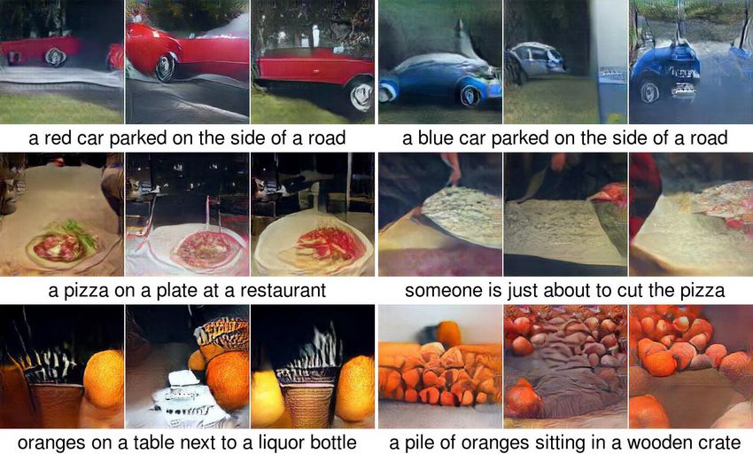
Generative Modeling
•   Density estimation

•   Sample generation

       Training examples   Model samples   (Goodfellow 2016)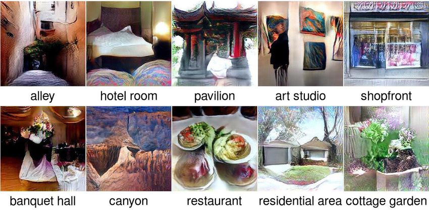
Roadmap
•   Why study generative modeling?

•   How do generative models work? How do GANs compare to
    others?

•   How do GANs work?

•   Tips and tricks

•   Research frontiers

•   Combining GANs with other methods
                                                       (Goodfellow 2016)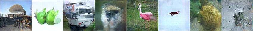
Why study generative models?
•   Excellent test of our ability to use high-dimensional,
    complicated probability distributions

•   Simulate possible futures for planning or simulated RL

•   Missing data

    •   Semi-supervised learning

•   Multi-modal outputs

•   Realistic generation tasks
                                                             (Goodfellow 2016)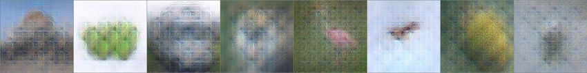
Next Video Frame Prediction
CHAPTER 15. REPRESENTATION LEARNING

             Ground Truth                    MSE                   Adversarial

Figure 15.6: Predictive generative networks provide an example of the importance of
learning which features are salient. In this example, the predictive generative network
has been trained to predict the appearance of a 3-D model of a human head at a specific
viewing angle. (Left)Ground truth. This is the correct image, that the network should
emit. (Center)Image produced by a predictive generative network trained with mean
                                (Lotter   et  al 2016)
squared error alone. Because the ears do not cause an extreme difference in brightness
                                                                               (Goodfellow 2016)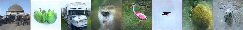
Single Image Super-Resolution

         (Ledig et al 2016)
                              (Goodfellow 2016)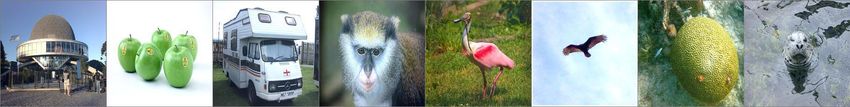
iGAN

    youtube

(Zhu et al 2016)   (Goodfellow 2016)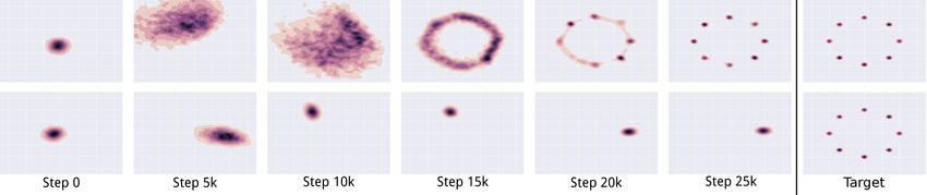
Introspective Adversarial
        Networks

            youtube

       (Brock et al 2016)   (Goodfellow 2016)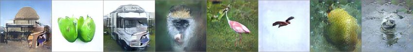
Phillip Isola                Jun-Yan Zhu                  Tinghui Zhou                    Alexei A. Efros

        Image to Image Translation            Berkeley AI Research (BAIR) Laboratory
                                                 University of California, Berkeley
                                    {isola,junyanz,tinghuiz,efros}@eecs.berkeley.edu
                                                                                           Figure 13: Example results of our method on day!night, co

                                                                             Input             Ground truth          Output                   Input
                    Labels to Street Scene                               Labels to Facade                                 BW to Color

            input                            output
                        Aerial to Map

                                                                     input                 output                 input                   output
                                                                                Day to Night                                 Edges to Photo

           input                             output                   input                     output               input                 output

Figure 1: Many problems in image processing, graphics, and vision involve translating an input image into a corresponding output im
These problems are often treated with application-specific algorithms, even though the setting is always the same: map pixels to p
Conditional adversarial nets are a general-purpose solution that appears Figure
                                                                         to work14: well on results
                                                                                    Example  a wide of variety of on
                                                                                                       our method these  problems.
                                                                                                                     automatically     Hereedges
                                                                                                                                   detected  we
                                                      (Isola et al 2016)
results of the method on several. In each case we use the same architecture and objective, and simply train on different data.
                                                                                                                                   (Goodfellow 2016)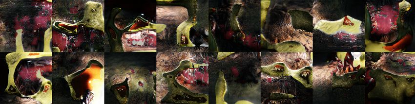
Roadmap
•   Why study generative modeling?

•   How do generative models work? How do GANs compare to
    others?

•   How do GANs work?

•   Tips and tricks

•   Research frontiers

•   Combining GANs with other methods
                                                       (Goodfellow 2016)
Maximum Likelihood
BRIEF ARTICLE
THE AUTHOR
✓ ⇤ = arg max Ex⇠pdata log pmodel (x | ✓)
✓
(Goodfellow 2016)Taxonomy of Generative Models
…
Direct
Maximum Likelihood
GAN
Explicit density Implicit density
Markov Chain
Tractable density Approximate density
-Fully visible belief nets GSN
-NADE
-MADE Variational Markov Chain
-PixelRNN Variational autoencoder Boltzmann machine
-Change of variables
models (nonlinear ICA) (Goodfellow 2016)Fully✓ =Visible
m likelihood
⇤
arg max E
Belief
log p
Nets
(x | ✓)
x⇠pdata model
✓
• Explicit formula based on chain (Frey et al, 1996)
ble belief net
rule: n
Y
pmodel (x) = pmodel (x1 ) pmodel (xi | x1 , . . . , xi 1 )
i=2
• Disadvantages:
• O(n) sample generation cost
PixelCNN elephants
• Generation not controlled by a
(van den Ord et al 2016)
latent code
(Goodfellow 2016)WaveNet
Amazing quality
Two minutes to synthesize
Sample generation slow
one second of audio
(Goodfellow 2016)visible belief net
n
Y
Change of Variables
pmodel (x) = pmodel (x1 ) pmodel (xi | x1 , . . . , xi 1)
i=2
e of variables
✓ ◆
@g(x)
y = g(x) ) px (x) = py (g(x)) det
@x
e.g. Nonlinear ICA (Hyvärinen 1999)
Disadvantages:
- Transformation must be
invertible
- Latent dimension must
match visible dimension
64x64 ImageNet Samples
Real NVP (Dinh et al 2016)
(Goodfellow 2016)of variables
✓ ◆
@g(x)
Variational Autoencoder
y = g(x) ) px (x) = py (g(x)) det
@x
nal (Kingma
bound and Welling 2013, Rezende et al 2014)
z log p(x) log p(x) DKL (q(z)kp(z | x))
=Ez⇠q log p(x, z) + H(q)
Disadvantages:
x -Not asymptotically
consistent unless q is
perfect
-Samples tend to have lower
quality
CIFAR-10 samples
(Kingma et al 2016) (Goodfellow 2016)log p(x) log p(x) DKL (q(z)kp(z | x))
=Ez⇠q log p(x, z) + H(q)
Machines Boltzmann Machines
1
p(x) = exp ( E(x, z))
Z
XX
Z= exp ( E(x, z))
x z
• Partition function is intractable
• May be estimated with Markov chain methods
• Generating samples requires Markov chains too
(Goodfellow 2016)GANs
• Use a latent code
• Asymptotically consistent (unlike variational
methods)
• No Markov chains needed
• Often regarded as producing the best samples
• No good way to quantify this
(Goodfellow 2016)Roadmap
• Why study generative modeling?
• How do generative models work? How do GANs compare to
others?
• How do GANs work?
• Tips and tricks
• Research frontiers
• Combining GANs with other methods
(Goodfellow 2016)Adversarial Nets Framework
D tries to make
D(G(z)) near 0,
D(x) tries to be G tries to make
near 1 D(G(z)) near 1
Differentiable
D
function D
x sampled from x sampled from
data model
Differentiable
function G
Input noise z
(Goodfellow 2016)x z
Generator Network
(G)
x = G(z; ✓ )
z
-Must be differentiable
- No invertibility requirement
- Trainable for any size of z
x
- Some guarantees require z to have higher
dimension than x
- Can make x conditionally Gaussian given z but
need not do so
(Goodfellow 2016)Training Procedure
• Use SGD-like algorithm of choice (Adam) on two
minibatches simultaneously:
• A minibatch of training examples
• A minibatch of generated samples
• Optional: run k steps of one player for every step of
the other player.
(Goodfellow 2016)Z= exp ( E(x, z))
x z
equation
Minimax
x = G(z; ✓ Game
) (G)
(D) 1 1
J = Ex⇠pdata log D(x) Ez log (1 D (G(z)))
2 2
(G) (D)
J = J
-Equilibrium is a saddle point of the discriminator loss
-Resembles Jensen-Shannon divergence
-Generator minimizes the log-probability of the discriminator
being correct
(Goodfellow 2016)Z= exp ( E(x, z))
x z
equation
Exercise
x = G(z; ✓ ) 1 (G)
(D) 1 1
J = Ex⇠pdata log D(x) Ez log (1 D (G(z)))
2 2
(G) (D)
J = J
• What is the solution to D(x) in terms of pdata and
pgenerator?
• What assumptions are needed to obtain this
solution?
(Goodfellow 2016)Solution
• Assume both densities are nonzero everywhere
• If not, some input values x are never trained, so
some values of D(x) have undetermined behavior.
• Solve for where the functional derivatives are zero:
(D)
J =0
D(x)
(Goodfellow 2016)p(x) = p(x | h)p(h)
maintains samples from a Markov chain from one learning step to the next in order
h
in a Markov chain as part of the inner loop of learning. The procedure is formally pr
Discriminator Strategy
ithm 1.
ce, equation 1 may not provide sufficient gradient for G to learn well. Early in l
is poor, D can reject samples with high confidence because they are clearly differe
ing data. Optimal
In this case,
D(x)log(1
for any D(G(z))) saturates.
pdata (x) and pmodel (x)Rather than training G to m
is always
D(G(z))) we can train G to maximize log D(G(z)). This(x)
pdata objective function resul
ed point of the dynamics of G and D(x) =
D but provides much stronger gradients early in l
pdata (x) + pmodel (x)
Discriminator Data
Model
Estimating this ratio distribution
using supervised learning is ...
the key approximation x
mechanism used by GANs
1
z
(a) (b) (c) (d)
(Goodfellow 2016)(D)
J = Ex⇠pdata log D(x) Ez log (1 D (G(z)))
2 2
(G) (D)
J = J
ng
Non-Saturating Game
(D) 1 1
J = Ex⇠pdata log D(x) Ez log (1 D (G(z)))
2 2
(G) 1
J = Ez log D (G(z))
2
-Equilibrium no longer describable with a single loss
-Generator maximizes the log-probability of the discriminator
being mistaken
1
-Heuristically motivated; generator can still learn even when
discriminator successfully rejects all generator samples
(Goodfellow 2016)DCGAN Architecture
Most “deconvs” are batch normalized
(Radford et al 2015)
(Goodfellow 2016)DCGANs for LSUN Bedrooms
(Radford et al 2015)
(Goodfellow 2016)Vector Space Arithmetic
CHAPTER 15. REPRESENTATION LEARNING
- + =
Man Man Woman
with glasses
Figure 15.9:
Woman with Glasses
A generative model has learned a distributed representation that disentangl
he concept of gender from the concept of wearing glasses. If we begin with the repr
(Radford
entation of the concept of a man et al,
with glasses, 2015)
then subtract the vector representing th
oncept of a man without glasses, and finally add the vector representing the conce
f a woman without glasses, we obtain the vector representing the concept of(Goodfellow
a woma 2016)Is the divergence important?
q ⇤ = argminq DKL (p q) q ⇤ = argminq DKL (q p)
p(x) p(x)
Probability Density
Probability Density
q ⇤ (x) q ⇤ (x)
x x
Maximum likelihood Reverse KL
ure 3.6: The KL divergence is asymmetric. Suppose we have a distribution p(x) a
(Goodfellow
to approximate it with another et q(x).
distribution al 2016)
We have the choice of minimiz
er DKL (pkq) or DKL (qkp). We illustrate the effect of this choice using a(Goodfellow
mixture 2016)Modifying GANs to do
Maximum Likelihood
THE AUTHOR
kelihood Non-saturating
(D) 1 1
J = Ex⇠pdata log D(x) Ez log (1 D (G(z)))
2 2
(G) 1 1
J = Ez exp (D (G(z)))
2
When discriminator is optimal, the generator
gradient matches that of maximum likelihood
(“On Distinguishability Criteria for Estimating Generative
Models”, Goodfellow 2014, pg 5) (Goodfellow 2016)Reducing GANs to RL
• Generator makes a sample
• Discriminator evaluates a sample
• Generator’s cost (negative reward) is a function of D(G(z))
• Note that generator’s cost does not include the data, x
• Generator’s cost is always monotonically decreasing in D(G(z))
• Different divergences change the location of the cost’s fastest
decrease
(Goodfellow 2016)Comparison of Generator Losses
5
0
5
J (G)
10
Minimax
15 Non-saturating heuristic
Maximum likelihood cost
20
0.0 0.2 0.4 0.6 0.8 1.0
D(G(z))
(Goodfellow 2014) (Goodfellow 2016)Loss does not seem to explain
why GAN samples are sharp
KL
Reverse
KL
(Nowozin et al 2016) KL samples from LSUN
Takeaway: the approximation strategy
matters more than the loss (Goodfellow 2016)Comparison to NCE, MLE
V (G, D) = Epdata log D(x) + Epgenerator (log (1 D(x)))
NCE
(Gutmann and MLE GAN
Hyvärinen 2010)
pmodel (x) Neural
D D(x) =
pmodel (x) + pgenerator (x) network
Goal Learn pmodel Learn pgenerator
None (G is Copy pmodel Gradient
G update rule
fixed) parameters descent on V
D update rule Gradient ascent on V
(“On Distinguishability Criteria…”, Goodfellow 2014) (Goodfellow 2016)Roadmap
• Why study generative modeling?
• How do generative models work? How do GANs compare to
others?
• How do GANs work?
• Tips and tricks
• Research frontiers
• Combining GANs with other methods
(Goodfellow 2016)Labels improve subjective
sample quality
• Learning a conditional model p(y|x) often gives much
better samples from all classes than learning p(x) does
(Denton et al 2015)
• Even just learning p(x,y) makes samples from p(x) look
much better to a human observer (Salimans et al 2016)
• Note: this defines three categories of models (no labels,
trained with labels, generating condition on labels)
that should not be compared directly to each other
(Goodfellow 2016)One-sided label smoothing
• Default discriminator cost:
cross_entropy(1., discriminator(data))
+ cross_entropy(0., discriminator(samples))
• One-sided label smoothed cost (Salimans et al
2016):
cross_entropy(.9, discriminator(data))
+ cross_entropy(0., discriminator(samples))
(Goodfellow 2016)Do not smooth negative labels
cross_entropy(1.-alpha, discriminator(data))
+ cross_entropy(beta, discriminator(samples))
Reinforces current generator behavior
(1 ↵)pdata (x) + pmodel (x)
D(x) =
pdata (x) + pmodel (x)
(Goodfellow 2016)Benefits of label smoothing
• Good regularizer (Szegedy et al 2015)
• Does not reduce classification accuracy, only confidence
• Benefits specific to GANs:
• Prevents discriminator from giving very large
gradient signal to generator
• Prevents extrapolating to encourage extreme samples
(Goodfellow 2016)Batch Norm
(1) (2) (m)
• Given inputs X={x , x , .., x }
• Compute mean and standard deviation of features of X
• Normalize features (subtract mean, divide by standard deviation)
• Normalization operation is part of the graph
• Backpropagation computes the gradient through the
normalization
• This avoids wasting time repeatedly learning to undo the
normalization
(Goodfellow 2016)Batch norm in G can cause
strong intra-batch correlation
(Goodfellow 2016)Reference Batch Norm
(1) (2) (m)
• Fix a reference batch R={r , r , .., r }
(1) (2) (m)
• Given new inputs X={x , x , .., x }
• Compute mean and standard deviation of features of R
• Note that though R does not change, the feature values change
when the parameters change
• Normalize the features of X using the mean and standard deviation
from R
(i)
• Every x is always treated the same, regardless of which other
examples appear in the minibatch
(Goodfellow 2016)Virtual Batch Norm
• Reference batch norm can overfit to the reference batch. A partial solution
is virtual batch norm
(1) (2) (m)
• Fix a reference batch R={r , r , .., r }
(1) (2) (m)
• Given new inputs X={x , x , .., x }
(i)
• For each x in X:
(i)
• Construct a virtual batch V containing both x and all of R
• Compute mean and standard deviation of features of V
(i)
• Normalize the features of x using the mean and standard deviation
from V
(Goodfellow 2016)Balancing G and D
• Usually the discriminator “wins”
• This is a good thing—the theoretical justifications are based on
assuming D is perfect
• Usually D is bigger and deeper than G
• Sometimes run D more often than G. Mixed results.
• Do not try to limit D to avoid making it “too smart”
• Use non-saturating cost
• Use label smoothing
(Goodfellow 2016)Roadmap
• Why study generative modeling?
• How do generative models work? How do GANs compare to
others?
• How do GANs work?
• Tips and tricks
• Research frontiers
• Combining GANs with other methods
(Goodfellow 2016)Non-convergence
• Optimization algorithms often approach a saddle
point or local minimum rather than a global
minimum
• Game solving algorithms may not approach an
equilibrium at all
(Goodfellow 2016)Exercise 2
• For scalar x and y, consider the value function:
V (x, y) = xy
• Does this game have an equilibrium? Where is it?
• Consider the learning dynamics of simultaneous
gradient descent with infinitesimal learning rate
(continuous time). Solve for the trajectory followed
by these dynamics.
@x @
= V (x(t), y(t))
@t @x
@y @
= V (x(t), y(t))
@t @y (Goodfellow 2016)Solution
This is the canonical example of
a saddle point.
There is an equilibrium, at
x = 0, y = 0.
(Goodfellow 2016)Solution
• The gradient dynamics are:
@x
= y(t)
@t
@y
= x(t)
@t
• Differentiating the second equation, we obtain:
2
@ y @x
2
= = y(t)
@t @t
• We recognize that y(t) must be a sinusoid
(Goodfellow 2016)Solution
• The dynamics are a circular orbit:
x(t) = x(0) cos(t) y(0) sin(t)
y(t) = x(0) sin(t) + y(0) cos(t)
Discrete time
gradient descent
can spiral
outward for large
step sizes
(Goodfellow 2016)Non-convergence in GANs
• Exploiting convexity in function space, GAN training is theoretically
guaranteed to converge if we can modify the density functions directly,
but:
• Instead, we modify G (sample generation function) and D (density
ratio), not densities
• We represent G and D as highly non-convex parametric functions
• “Oscillation”: can train for a very long time, generating very many
different categories of samples, without clearly generating better samples
• Mode collapse: most severe form of non-convergence
(Goodfellow 2016)Mode Collapse
min max V (G, D) 6= max min V (G, D)
G D D G
• D in inner loop: convergence to correct distribution
Under review as a conference paper at ICLR 2017
• G in inner loop: place all mass on most likely point
AN training on a toy 2D mixture of Gaussians
distribution after increasing numbers of training
n. The top row shows training for a GAN with
(Metz
ut and converges to the target et al 2016)
distribution. The (Goodfellow 2016)Reverse KL loss does not
explain mode collapse
• Other GAN losses also yield mode collapse
• Reverse KL loss prefers to fit as many modes as the
model can represent and no more; it does not prefer
fewer modes in general
• GANs often seem to collapse to far fewer modes
than the model can represent
(Goodfellow 2016)waran Mode collapse causes low
REEDSCOT 1 , AKATA 2 , XCYAN 1 , LLAJAN 1
SCHIELE 2 , HONGLAK 1
MPI - INF. MPG . DE)
output diversity
this small bird has a pink this magnificent fellow is
breast and crown, and black almost all black with a red
primaries and secondaries. crest, and white cheek patch.
the flower has petals that this white and yellow flower
are bright pinkish purple have thin white petals and a
with white stigma round yellow stamen
(Reed et al, submitted to
ICLR 2017)
Figure 1. Examples of generated images from text descriptions.
(Reed et al 2016)
Left: captions are from zero-shot (held out) categories, unseen
ext. Right: captions are from the training set.
properties of attribute representations are attractive, at-
ributes are also cumbersome to obtain as they may require
domain-specific knowledge. In comparison, natural lan- (Goodfellow 2016)Minibatch Features
• Add minibatch features that classify each example
by comparing it to other members of the minibatch
(Salimans et al 2016)
• Nearest-neighbor style features detect if a minibatch
contains samples that are too similar to each other
(Goodfellow 2016)Minibatch GAN on CIFAR
Training Data Samples
(Salimans et al 2016) (Goodfellow 2016)Minibatch GAN on ImageNet
(Salimans et al 2016) (Goodfellow 2016)Cherry-Picked Results
(Goodfellow 2016)Problems with Counting
(Goodfellow 2016)Problems with Perspective
(Goodfellow 2016)Problems with Global
Structure
(Goodfellow 2016)This one is real
(Goodfellow 2016)Unrolled GANs
Under review as a conference paper at ICLR 2017
Under review as a conference paper at ICLR 2017
• Backprop through k updates of the discriminator to
prevent mode collapse:
(Metz et al 2016)
Figure 1: Unrolling the discriminator stabilizes GAN training on a toy 2D mixture of Gau
dataset. Columns show a heatmap of the generator distribution after increasing numbers of tr
steps. The final column shows the data distribution. The top row shows training for a GAN
10 unrolling
Figure steps. Itsthe
1: Unrolling generator quicklystabilizes
discriminator spreads out
GAN andtraining
converges
on to the 2D
a toy target distribution
mixture of G
bottom row
dataset. showsshow
Columns standard GAN of
a heatmap training. The generator
the generator rotates
distribution afterthrough the modes
increasing numbers of of th
steps. The final column shows the data distribution. The top row shows training for ama
distribution. It never converges to a fixed distribution, and only ever assigns significant
(Goodfellow 2016)
GAEvaluation
• There is not any single compelling way to evaluate a generative
model
• Models with good likelihood can produce bad samples
• Models with good samples can have bad likelihood
• There is not a good way to quantify how good samples are
• For GANs, it is also hard to even estimate the likelihood
• See “A note on the evaluation of generative models,” Theis et al
2015, for a good overview
(Goodfellow 2016)Discrete outputs
• G must be differentiable
• Cannot be differentiable if output is discrete
• Possible workarounds:
• REINFORCE (Williams 1992)
• Concrete distribution (Maddison et al 2016) or Gumbel-
softmax (Jang et al 2016)
• Learn distribution over continuous embeddings, decode to
discrete
(Goodfellow 2016)Supervised Discriminator
Real
Real Fake Real cat Fake
dog
Hidden Hidden
units units
Input Input
(Odena 2016, Salimans et al 2016) (Goodfellow 2016)). By using minibatch discrimination
ection 3.2) we can improve their visual quality. On MTurk, annotators were a
amples in 52.4% of cases (2000 votes total), where 50% would be obtained b
Semi-Supervised Classification
Similarly, researchers in our institution were not able to find any artifacts that
to distinguish samples. However, semi-supervised learning with minibatch disc
roduce as good a classifier as does feature matching.
MNIST (Permutation Invariant)
Model Number of incorrectly predicted test examples
for a given number of labeled samples
20 50 100 200
DGN [21] 333 ± 14
Virtual Adversarial [22] 212
CatGAN [14] 191 ± 10
Skip Deep Generative Model [23] 132 ± 7
Ladder network [24] 106 ± 37
Auxiliary Deep Generative Model [23] 96 ± 2
Our model 1677 ± 452 221 ± 136 93 ± 6.5 90 ± 4.2
Ensemble of 10 of our models 1134 ± 445 142 ± 96 86 ± 5.6 81 ± 4.3
Number of incorrectly classified test examples for the semi-supervised setting on
ant MNIST. Results are averaged over 10 seeds.
AR-10
(Salimans et al 2016) (Goodfellow 2016)Ladder network [24] 106 ± 37
Auxiliary Deep Generative Model [23] 96 ± 2
Our model 1677 ± 452 221 ± 136 93 ± 6.5 90 ± 4.2
Ensemble of 10 of our models 1134 ± 445 142 ± 96 86 ± 5.6 81 ± 4.3
Semi-Supervised Classification
ber of incorrectly classified test examples for the semi-supervised setting on permuta-
MNIST. Results are averaged over 10 seeds.
-10 CIFAR-10
Model Test error rate for
a given number of labeled samples
1000 2000 4000 8000
Ladder network [24] 20.40±0.47
CatGAN [14] 19.58±0.46
Our model 21.83±2.01 19.61±2.09 18.63±2.32 17.72±1.82
Ensemble of 10 of our models 19.22±0.54 17.25±0.66 15.59±0.47 14.87±0.89
est error on semi-supervised CIFAR-10. Results are averaged over 10 splits of data.
SVHN
378 Model Percentage of incorrectly predicted test examples
a small, well studied
379dataset of 32 ⇥ 32 natural images. We use for this datanumber
a given set to studysamples
of labeled
ed learning, as well as to examine the visual quality of samples500that can be 1000 achieved. 2000
380
minator in our GAN we use a 9 layer deep convolutional network with36.02±0.10
DGN [21] dropout and
381
alization. The generator is a 4 layer deep
Virtual CNN[22]with batch normalization.24.63
Adversarial Table 2
382
ur results on the semi-supervised learning
Auxiliary task. Model [23]
Deep Generative 22.86
Skip Deep Generative Model [23] 16.61±0.24
383 Our model 18.44 ± 4.8 8.11 ± 1.3 6.16 ± 0.58
384 Ensemble of 10 of our models
6
5.88 ± 1.0
385
(Salimans et al
Figure 5: (Left) 2016)
Error rate on SVHN. (Right) Samples fro (Goodfellow 2016)Learning interpretable latent codes /
controlling the generation process
InfoGAN (Chen et al 2016) (Goodfellow 2016)RL connections
• GANs interpreted as actor-critic (Pfau and Vinyals
2016)
• GANs as inverse reinforcement learning (Finn et al
2016)
• GANs for imitation learning (Ho and Ermon 2016)
(Goodfellow 2016)Finding equilibria in games
• Simultaneous SGD on two players costs may not
converge to a Nash equilibrium
• In finite spaces, fictitious play provides a better
algorithm
• What to do in continuous spaces?
• Unrolling is an expensive solution; is there a
cheap one?
(Goodfellow 2016)Other Games in AI
• Board games (checkers, chess, Go, etc.)
• Robust optimization / robust control
• for security/safety, e.g. resisting adversarial examples
• Domain-adversarial learning for domain adaptation
• Adversarial privacy
• Guided cost learning
• …
(Goodfellow 2016)Exercise 3
• In this exercise, we will derive the maximum likelihood cost for
GANs.
• We want to solve for f(x), a cost function to be applied to every
sample from the generator:
J (G) = Ex⇠pg f (x)
• Show the following:
@ (G) @
J = Ex⇠pg f (x) log pg (x)
@✓ @✓
• What should f(x) be?
(Goodfellow 2016)Solution
@ (G) @
• To show that J = Ex⇠pg f (x) log pg (x)
@✓ @✓
• Expand the expectation to an integral
Z
@ @
Ex⇠pg f (x) = pg (x)f (x)dx
@✓ @✓
• Assume that Leibniz’s rule may be used
Z
@
f (x) pg (x)dx
@✓
• Use the identity
@ @
pg (x) = pg (x) log pg (x)
@✓ @✓ (Goodfellow 2016)Solution
@ (G) @
• We now know J = Ex⇠pg f (x) log pg (x)
@✓ @✓
• The KL gradient is Ex⇠pdata @
log pg (x)
@✓
• We can do an importance sampling trick
pdata (x)
f (x) =
pg (x)
• Note that we must copy the density pg or the
derivatives will double-count
(Goodfellow 2016)Solution
pdata (x)
• We want f (x) = pg (x)
pdata (x)
• We know that D(x) = (a(x)) =
pdata (x) + pg (x)
• By algebra f (x) = exp(a(x))
(Goodfellow 2016)Roadmap
• Why study generative modeling?
• How do generative models work? How do GANs
compare to others?
• How do GANs work?
• Tips and tricks
• Combining GANs with other methods
(Goodfellow 2016)Plug and Play Generative
Models
• New state of the art generative model (Nguyen et al
2016) released days before NIPS
• Generates 227x227 realistic images from all
ImageNet classes
• Combines adversarial training, moment matching,
denoising autoencoders, and Langevin sampling
(Goodfellow 2016)oming Geometric Intelligence Montreal Institute for Learning Algorithms
l.com jason@geometric.ai yoshua.umontreal@gmail.com
Alexey Dosovitskiy Jeff Clune
University of Freiburg
osovits@cs.uni-freiburg.de PPGN Samples University of Wyoming
jeffclune@uwyo.edu
stract
on, photo-realistic images has
n machine learning. Recently,
ne interesting way to synthesize
g gradient ascent in the latent
rk to maximize the activations
n a separate classifier network.
method by introducing an addi-
e, improving both sample qual-
ding to a state-of-the-art gen-
high quality images at higher
n previous generative models,
ageNet categories. In addition,
ilistic interpretation of related
hods and call the general class
Generative Networks.” PPGNs
ator network G that is capable
image types and 2) a replace-
C that tells the generator what
e generation of images condi-
s an ImageNet or MIT Places
also conditioned on a caption (Nguyen et al 2016)
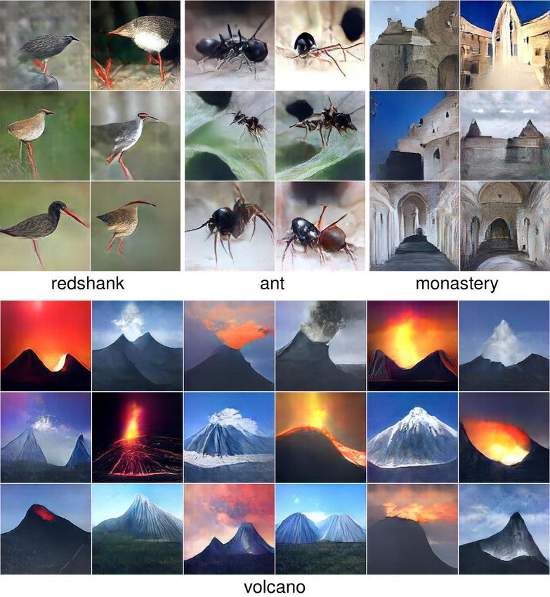
Figure 1: Images synthetically generated by Plug and Play
(Goodfellow 2016)
ing network). Our method also Generative Networks at high-resolution (227x227) for fourPPGN for caption to image
Figure 5:(Nguyen
Images synthesized to
et al 2016) (Goodfellow 2016)Basic idea
• Langevin sampling repeatedly adds noise and
gradient of log p(x,y) to generate samples (Markov
chain)
• Denoising autoencoders estimate the required
gradient
• Use a special denoising autoencoder that has been
trained with multiple losses, including a GAN loss,
to obtain best results
(Goodfellow 2016)Sampling without class
gradient
(Nguyen et al 2016) (Goodfellow 2016)GAN(a)loss
(b)
is
Joint
Real
a key
PPGN-h (L
images
ingredient
+L +L +L
img h1 h
Raw data Reconstruction Reconstruction
alJoint
images
PPGN-h (Limg(c)+LLGAN
h1 +removed
Lh + LGAN (Limg) + Lh1 + L
by PPGN by PPGN
without GAN
Images from Nguyen et al 2016
First observed by Dosovitskiy et al 2016 (Goodfellow 2016)Conclusion
• GANs are generative models that use supervised learning to
approximate an intractable cost function
• GANs can simulate many cost functions, including the one
used for maximum likelihood
• Finding Nash equilibria in high-dimensional, continuous, non-
convex games is an important open research problem
• GANs are a key ingredient of PPGNs, which are able to
generate compelling high resolution samples from diverse
image classes
(Goodfellow 2016)You can also read