Grappling with the New Reality of Zero Bond Yields Virtually Everywhere - JULY 2020
←
→
Page content transcription
If your browser does not render page correctly, please read the page content below
Grappling with the New Reality of
Zero Bond Yields Virtually Everywhere
JULY 2020

© 2020 Bridgewater Associates, LP
Part 1:
The Facts and the Implications
JULY 13, 2020

BOB PRINCE
GREG JENSEN
MELISSA SAPHIER

© 2020 Bridgewater Associates, LP
I
     t is now a reality that long-term bond yields are at or near zero in the US
     and virtually everywhere. There are so many implications of this that it
     takes some time to recognize and absorb them all and then more time to
work through what to do about it, which is what we’ve been doing and what
we see the biggest and most sophisticated institutional investors doing as
well. Given the status of the US dollar as the primary reserve currency and US
bonds as the “risk-free asset,” having the US bond yield at or near zero goes
beyond the implications for bonds the asset because the interest rate is the
price of credit and is the discount rate on all other cash flows. A zero interest
rate effectively means that there is no interest rate, and if it stays at zero, it
means no change in the interest rate. Thus, any asset or any form of credit that
is impacted by the level or the change in the interest rate is impacted, which
extends to all economies and markets and the policies that drive them.

For us to say that we are here is something, since, as you know, we’ve explained for a decade or more why low
bond yields are not really a problem, and during this time, we’ve put low bond yields to good use in beta and in
alpha. But we’ve now crossed a line, and we all have to deal with this new reality.

Among the questions that this raises are the following:

     •    How much room is left for bonds to rally?

     •    What is the potential to earn a risk premium by holding leveraged bonds funded by cash?

     •    What are the asymmetries pertaining to the range of potential bond returns?

     •    For portfolios that include equities and bonds, how much support is lost from bonds no longer being
          able to cushion a decline in equities?

     •    How does the downside of equities and other assets change if the discount rate on cash flows can’t fall?

     •    For the economy and earnings, how does this impact the ability to cushion or pull out of a downturn?

     •    How does this impact the operation of monetary and fiscal policy?

     •    What are the portfolio implications, and what can be done to make portfolios more resilient?

Given such questions, in one way or another, the zero bond yield has been the gravitational center of our
research in recent months, and we’ve both made adjustments and developed new insights related to it. The
purpose of this research paper is to walk through some of this. The topics are obviously deep and complex.
In Part 1, we will just touch on these questions and then in Parts 2 and 3 get into the what-do-you-do-about-
it. Before we go to the specifics, the following chart showing US bond yields since 1800 starts to convey the
uniqueness of the current circumstances.

© 2020 Bridgewater Associates, LP                                                                                3
USA Nominal 10yr Bond Yield
18%
16%
14%
12%
10%
8%
6%
4%
2%
0%
1800 1820 1840 1860 1880 1900 1920 1940 1960 1980 2000 2020
The Uniqueness of a Zero Bond Yield and No Risk
Premium/Yield Curve Slope versus Cash
Not only is the bond yield lower than ever, this is the first time it’s been low with a flat yield curve. For example, in 2009
when the short-term interest rate was zero, the yield curve slope was about 3%, and in 1933 when short rates were zero
and the Fed started printing, the bond yield was 3.5%. So in those cases, even though yields were low and the long-
term expected return of holding bonds was similarly low, the potential for excess returns in leveraged bonds was very
high due to the implied rise in bond yields as reflected in those steep yield curves and the long duration of the bonds.
Today, we have long durations but little or no rise priced in, little or no risk premium versus cash, and obviously a low
expected total return of holding those bonds.
Long Rate Short Rate
20%
18%
16%
14%
12%
10%
8%
6%
4%
2%
0%
-2%
1900 1910 1920 1930 1940 1950 1960 1970 1980 1990 2000 2010 2020
© 2020 Bridgewater Associates, LP 4For additional perspective, the table below shows bond returns during a couple periods of zero short-term
interest rates as well as projections based on today’s pricing. In past cases, there was a chance to accrue a
higher starting forward yield and to benefit as yields gradually drifted down. Today, we have a lower starting
point and less opportunity for yields to decline relative to what is discounted to further boost returns. Below,
we show returns over the next three years if yields were to fall to zero or all the way to an extreme of -1%.
1934–1947 End of 2008 Next 3 Years Next 3 Years
to Today If Rates Fall to 0% If Rates Fall to -1%
Short Rate at Start of Period 0.2% 0.0% 0.1% 0.1%
Total Annualized Returns 4.3% 4.1% 2.3% 5.3%
Starting Yield 3.2% 2.9% 0.6% 0.6%
Impact of Yield Changes 1.1% 1.1% 1.7% 4.7%
While one can’t say for sure how low yields could go, the obvious limitation is that at a certain level, cash
hoarding becomes a more attractive alternative. Given the frictions between the central bank policy rate and
the rates facing other borrowers and lenders (we would guess around -1%), policy rates would be unlikely to
trigger a move to cash in most countries. Below that point, it becomes less clear. And at least for now, central
bankers across the world have expressed growing hesitancy about further use of negative rates as a policy tool,
in particular focusing on the potential adverse effects for the banking system, which could weaken the efficacy
of such policies.
What are the asymmetries in the range of potential bond returns in this environment?
With limited room for yields to fall and no limit on how much they can rise, the distribution of potential
returns for bonds and rates is adversely skewed. Of course, looking back there are underlying secular forces
that have pulled yields down, and in practice, how yields evolve from here will depend on how economic
conditions unfold, how policy makers respond, and how that impacts investor preferences. Considering the
range of outcomes looking out over the next three years, a “best case” bond rally to -1% would bring bond
returns to a cumulative 17%. Whereas if we were to see real yields return to their long-term average (a little
over 2%) and a moderate rise in inflation to 4%, that would produce about -30% returns over the three years.
USA Nominal Bond Cumulative Total Returns over 3 Years in Different Scenarios
40%
30%
17% 20%
7%
3% 10%
0%
-10%
-20%
-19%
-30%
-31%
-40%
Yields Fall to -1% Yields Fall to Zero Yields Don’t Move LT Avg RY LT Avg RY
(Lowest Yield Globally) + Current BEI + 4% BEI
© 2020 Bridgewater Associates, LP 5How widespread are these conditions globally?
After this year’s bond rally, this problem is truly a global one. Roughly 80% of the market cap of local currency
government debt has a yield below 1%.
Percent of Bonds Yielding Below 1%
100%
90%
80%
70%
60%
50%
40%
30%
20%
10%
0%
2010 2012 2014 2016 2018 2020
For portfolios that include equities and bonds, how much support is lost from bonds no longer being
able to cushion a downturn? How does the downside of equities and other assets change if the discount
rate on cash flows can’t fall?
This year, we got a glimpse of what it looks like when bond yields are already floored when a downturn arrives.
While US bonds had room to fall and produce strong returns, there was much less support in Europe and none
in Japan.
Nominal Bond Cumulative Total Returns This Year
USA EUR JPN
10%
8%
6%
4%
2%
0%
-2%
Jan-20 Feb-20 Mar-20 Apr-20 May-20 Jun-20 Jul-20
© 2020 Bridgewater Associates, LP 6Normally when economic conditions are deteriorating and equities are falling, a bottom is formed when the
central bank steps in and provides enough easing to offset these negative pressures. This supports equities
in two ways: the support to the economy helps stabilize earnings prospects, and the declining discount rate
pushes up the present value of future earnings. Looking across the US bear markets of the past several decades
in the chart below, you can see how falling rates provided a cushion, especially when the Fed stepped in to
offset the more extreme cases. Allowing for a duration of perhaps 7 to 10 years, you can ballpark the price
impact of the decline in yields.
USA Equity Drawdowns Larger Than 20% since 1925
Max Decline in Interest Rates
Period Equity Drawdown Short Rates Long Rates
1929–1945 -84% -4.8% -2.6%
2007–2012 -52% -3.4% -2.6%
2000–2006 -46% -5.6% -2.5%
1973–1976 -43% -4.6% -0.9%
2020 -34% -1.5% -0.9%
1987–1989 -29% -0.6% -1.5%
1968–1971 -29% -5.0% -2.5%
1962–1963 -22% 0.0% -0.3%
1946–1949 -22% -0.1% -0.4%
Average -40% -2.9% -1.6%
For the economy and earnings, how does this impact the ability to cushion or pull out of a downturn?
In prior downturns, the Fed helped arrest the downturn and engineered a recovery by lowering rates an
average of 500bps. And in the financial crisis when they ran out of room to lower short rates, 500bps plus QE
helped lower longer-term yields. Now, with that room depleted, the task before policy makers is much tougher
and requires new policy tools, which we’ll discuss in depth in Part 2 of this series.
Fed Tightening Cycles
Fed Funds Rate Easing Tightening
20%
18%
16%
14%
12%
10%
8%
6%
4%
2%
0%
1920 1930 1940 1950 1960 1970 1980 1990 2000 2010 2020
© 2020 Bridgewater Associates, LP 7Fed Funds Rates*
Low Date Nominal Period % Change High Date
Change (in months)
3.96% Oct-19 1.92% 14 49% 5.88% Dec-20
-3.96% 43 -67%
1.92% Jul-24 2.88% 64 150% 4.80% Nov-29
-4.80% 34 -100%
0.00% Sep-32 2.09% 251 — 2.10% Aug-53
-1.44% 10 -69%
0.65% Jun-54 2.94% 40 452% 3.59% Oct-57
-2.71% 8 -75%
0.88% Jun-58 3.69% 18 419% 4.57% Dec-59
-2.30% 19 -50%
2.27% Jul-61 3.32% 62 146% 5.59% Sep-66
-2.26% 9 -40%
3.33% Jun-67 4.75% 30 143% 8.08% Dec-69
-4.08% 26 -50%
4.00% Feb-72 7.00% 28 175% 11.00% Jun-74
-6.25% 30 -57%
4.75% Dec-76 11.75% 39 247% 16.50% Mar-80
-5.50% 5 -33%
11.00% Apr-80 8.00% 9 73% 19.00% May-81
-11.00% 18 -58%
8.00% Nov-82 3.44% 21 43% 11.44% Sep-84
-5.56% 26 -49%
5.88% Oct-86 3.87% 31 66% 9.75% May-89
-6.75% 40 -69%
3.00% Sep-92 3.50% 99 117% 6.50% Dec-00
-5.50% 30 -85%
1.00% Jun-03 4.25% 50 425% 5.25% Aug-07
-5.25% 100 -100%
0.00–0.25% Dec-15 2.25% 43 — 2.25% Jul-19
-2.25% 7 -100%
*
Prior to 1975, T-bills used as proxy for Fed funds target rate
Avg Increase 4.38% 53
Range of Increases 1.9% to 11.8% 9 to 251
Avg Decrease -4.64% 27
Range of Decreases -11.0% to -1.4% 5 to 100
© 2020 Bridgewater Associates, LP 8Zero nominal yields also create a unique linkage between real yields and inflation. Because there is an arbitrage
between the breakeven inflation rate and actual inflation, a deflationary downturn that pushes breakeven
inflation down is extra risky because the combination pushes real yields up as the economy contracts (because
the real yield plus breakeven inflation must equal the nominal yield, and the nominal yield is relatively stable),
i.e., you have a higher discount rate on cash flows as cash flows fall. On the other hand, if reflation is successful,
central banks will likely delay the rise in nominal yields relative to inflation, forcing real yields to fall. And
there is no lower limit to either real yields or breakeven inflation. As a result, a successful reflation can drive
real yields much lower even if they start at low levels, and policy failure (i.e., deflation) will drive them higher.
As shown below, Japan has experienced these dynamics since the ’90s. Before rates reached the zero lower bound
(marked below with a gray vertical line), inflation and short rates fell and rose together, reflecting the central
bank’s responsiveness to conditions. But after rates reached zero, the relationship inverted. Falling inflation,
when rates are already at zero, forces real yields higher, producing a tightening as conditions are deteriorating.
Japan
Core Inflation (Y/Y) Real Short Rate
10% 10%
Inflation and real short rates Nominal rate hits zero
rising and falling together and relationship inverts
8% 8%
6% 6%
4% 4%
2% 2%
0% 0%
-2% -2%
-4% -4%
1985 1990 1995 2000 2005 2010 2015 2020
How to build a resilient portfolio in such a world?
We’ll share our thoughts on this below.
© 2020 Bridgewater Associates, LP 9Part 2: Achieving Balance in a “Monetary Policy 3” World JULY 14, 2020 GREG JENSEN BOB PRINCE © 2020 Bridgewater Associates, LP
I
    n Part 1 of this series, we laid out the problem that 0% bond yields
    presents for all investors. In Part 2, we explore how we are approaching
    this challenge in our own balanced portfolios; in Part 3 to follow, we
will approach the issue from the perspective of more traditional portfolios,
exploring more incremental steps toward improving diversification and
reducing portfolio vulnerabilities.

In terms of building a balanced strategic asset allocation, it is pretty obvious that with interest rates near zero
and being held stable by central banks, bonds can provide neither returns nor risk reduction. It is also true that
policy makers have had to move on in terms of their tools for dealing with downturns. Instead of interest rate
cuts, policy has moved to MP3 (i.e., the coordination of monetary and fiscal policy). Understanding the nature
of MP3 and how it will affect different asset classes allows us to logically balance assets for an MP3 world.

While the loss of nominal bonds as a source of return and diversification is a big deal for most asset allocations,
our balanced approach to beta has never been about a particular asset allocation, nor has it ever been reliant
on any particular asset class. Rather, it is an approach to getting the most out of the full menu of assets that are
available. Near-zero interest rates changes the menu of choices that one has available; it doesn’t change the
principles of asset pricing and balance. The two key building blocks of balance for us are:

              1.      Select assets that will outperform cash over time;
              2.      Diversify those assets based on how they will react to future economic scenarios.

As long as you can achieve 1 and 2, “balanced beta” is achievable, and we expect it will likely offer superior risk-
adjusted returns compared to typical portfolios. We believe we can achieve these conditions going forward by
taking the following steps:

       •      First, we are moving into alternatives to nominal bonds that we believe can balance equity risk in
              an MP3 world. In an MP3 world, policy makers will respond to a downturn through coordinated
              monetary and fiscal policy—putting money to work in the real economy, financed by money printing.
              If this does not succeed in reflating equities, logically we would expect this printed money to end up in
              inflation-hedge assets like inflation-linked bonds and gold. This has been borne out by our historical
              studies of reflations across time and economies. So while we continue to hold nominal bonds in markets
              where there is potential room for one more bond rally, we are increasingly using these inflation-hedge
              assets as well to get balance where we previously would have used nominal bonds.

       •      Second, we are bolstering our geographic diversification. The price of any asset, of any type, can be
              thought of as a stream of future cash flows discounted by a rate that includes the risk-free discount
              rate (the expected return of cash) and a risk premium. In a world in which risk-free discount rates
              are relatively stable, diversification of risk premiums and cash flows themselves takes on heightened
              importance. Cross-asset diversification can help with the cash flows, but assets within a region
              and, more generally, with similar investor bases tend to have highly related risk premiums, so
              historically it has been a challenge to diversify this risk. With the opening up of markets in China
              and the surrounding Asia bloc, a third pole of global importance comparable to the US and Europe
              has become available as a source of diversification. Different economic conditions, independent
              monetary policy, and distinct savings patterns mean risk premiums and cash flows in this third pole
              are lowly related to those in the developed world. Geographic diversification will likely be both more
              impactful and more needed going forward than it has been in recent decades, given the potential for
              de-globalization and increased fragmentation, if not outright conflict.

There is no guarantee expected performance can or will be achieved.

© 2020 Bridgewater Associates, LP                                                                                    11
• Third, we are exploring ways to structure an equities allocation to reduce the need for balancing
assets in the first place. By identifying specific types of demand and connecting those forms of
spending to the companies that receive that spending in the form of revenue, and then screening
for the quality of balance sheets and operating stability, we are able to hold a set of publicly traded
companies whose earnings we expect to approach the consistency of the coupon on a bond. We
believe these portfolios can serve as more stable storeholds of wealth than broad equities, reducing
(though not eliminating) the need to hold diversifying assets against them. Because for now this is
playing a relatively modest role in our own beta portfolios, we’ll save further discussion of the topic
for another time.
Below, we elaborate on how we are approaching balance in this environment; given the importance of the
topic, we are sharing our thinking in real time and will share more as our research progresses.
We Are Now in an MP3 World: Monetary and Fiscal Reflation
as the Tool to Stimulate
To us, the question of how to invest in a world with yields at zero is the question of how to invest in an MP3
world—a world in which interest rates (Monetary Policy 1/MP1) and quantitative easing (MP2) have been
exhausted as tools to stimulate, and coordinated monetary and fiscal stimulus (MP3) becomes the policy tool
of choice. The necessary shifts in the overarching policy regime are what have brought us here, and it was the
nature of the prevailing policy regime that was to a significant degree responsible for nominal bonds being
such a good diversifier to equities in the first place.
To briefly review, MP1 is interest rate policy—raising and lowering short-term interest rates to tighten and
ease monetary policy. That channel primarily affects borrowers, by raising or lowering borrowing costs across
the economy. When rates hit zero, the next step is MP2—quantitative easing, which targets savers. QE lifts
savers out of assets, with the hope that those savers will then invest in riskier assets (thus boosting asset prices
and stimulating spending through the wealth effect) or spend in the real economy. MP3 is fiscal spending
monetized by central bank printing, where the central bank effectively prints money and the government puts
it to work in the real economy.
Channels by Which MP1, MP2, and MP3 Stimulate Spending
Monetary Policy 1 Borrowers
(interest rate policy) (interest rate induced spending)
Monetary Policy 2 Savers
(QE) (asset/liquidity induced spending)
Monetary Policy 3 Government
(coordinated fiscal- (direct spending financed
monetary actions) by money printing)
The fact that MP1 and MP2 have been the operative policy paradigms has been a key reason why nominal
bonds have historically been such a good balancer of equities: the lever used by central banks to stimulate in
the event of a downturn was to lower interest rates (in the case of MP1) and then to buy assets and flatten yield
curves when short rates could be lowered no more (in the case of MP2). With short rates now zero and yield
curves essentially flat in most of the developed world, this dynamic is now behind us.
There is no guarantee expected performance can or will be achieved.
© 2020 Bridgewater Associates, LP 12The end of the prior policy paradigm and the shift to MP3 occurred in two steps: 1) the shift away from preemptive tightening following the Fed’s 2018 tightening; and 2) the exhaustion of interest rates and QE and the shift to coordinated monetary and fiscal policy in response to the global pandemic. It’s noteworthy that even with the 2008 shift toward QE, the inflation-fighting mentality of the Volcker era was still in the background until very recently, with the Fed raising rates at the end of 2018 based on cyclical conditions. We think that was the last preemptive tightening we will see for some time. Given the outsize impact that tightening had on the economy and assets, central banks very quickly changed their tune, with every major developed world central bank making it clear that they will wait for substantially higher-than-target inflation for a significant period before tightening policy. 2019 was then a transition year, with no more preemptive tightening but some small room left in MP1 and MP2. The virus shock required central banks to spend that remaining fuel essentially all at once, with the need for direct fiscal stimulus at the same time as “whatever it takes”/unlimited QE signaling the dawn of MP3. 1940s US Wartime Policy Helps Illustrate MP3 Mechanics: Pegged Yields; Reflation Through Money Printing and Fiscal; Inflation Much Higher Than Bond Yields We are still early in the MP3 era, with many open questions about what form it will take and a high likelihood it will evolve over time through experimentation. But the yield curve targeting environment of the 1940s in the US is a good case study on what such policies can look like. The period has rather striking parallels to present circumstances—the end of a long-term debt cycle, a relatively modest cyclical tightening leading to a big economic and market decline, an abrupt policy reversal, and then the need for a new form of policy to finance a massive fiscal expansion once interest rates and QE have been exhausted. And as described in our June 23 research, the Fed is explicitly considering yield curve targeting, with many market participants expecting the Fed to announce a front-end target later in the year. In the aftermath of the Great Depression and after a tightening of monetary and fiscal policy in 1937 that led to a collapse in growth and equities, the US pinned yields at low levels and printed significant quantities of money to fund the growing wartime fiscal deficit. You can see both how bonds behaved and how stimulation worked during this period of “wartime MP3” in the charts below. Short rates were kept near zero and long rates were pegged slightly higher to maintain a fairly steep yield curve (to ensure a low but steady return to bondholders). But rates did not move at all with cyclical conditions (growth and inflation), meaning bonds would have provided no diversification benefit. Rather, the Fed expanded and contracted the monetary base to manage the cycle, with a big upward trend to finance the deficit. Notably, inflation rose significantly above the bond yield in the early and then late ‘40s, well into double digits, which had the beneficial effect of inflating away nominal debts. © 2020 Bridgewater Associates, LP 13
1930s–1940s
                                                                                                Government Spending Total (%GDP)
             Interest Rates            Monetary Base (%GDP)                                     of which Direct Spending
7%                                                                 18%                                                                           40%
                                                                                                      WWII
6%                    Money supply becomes                                                                                                       35%
                      the monetary lever                           16%
                                                                            Monetized
                                                                            fiscal                                                               30%
5%
                                                                   14%      expansion
                                                                                                                                                 25%
4%
                                                                   12%                                                                           20%
3%
                                                                                                                                                 15%
                                                                   10%          New Deal
2%
                                                                                                                                                 10%
                                    Pegged short rate              8%
1%                                                                                                                                               5%

0%                                                                 6%                                                                            0%
     25         30            35          40            45                 30            40            50           60          70          80

                          Bond Yield              Growth                                               Bond Yield          Inflation
                                                                   30%                                                                           30%

                                                                                                                                                 25%
                                                                   20%                                  Inflation much higher
                                                                                                        than bond yield
                                                                                                                                                 20%

                                                                   10%
                                                                                                                                                 15%

                                                                                 Pegged long rate,                                               10%
                                                                   0%
                                                                                 volatile inflation
                              Pegged long rate,
                              volatile growth                                                                                                    5%
                                                                   -10%
                                                                                                                                                 0%

                                                                   -20%                                                                          -5%
     35    37        39        41       43        45         47            35         37        39           41     43          45     47

While MP3 in today’s world might look significantly different than how policy makers managed the ‘40s,
the basic elements of highly managed and near-zero rates, money printing to fund fiscal deficits, and higher
inflation being tolerated if not desired given high debt levels are very likely going forward. And some have
argued explicitly that exceptional “wartime” policies like what we saw in the ‘40s are called for in the face of
the ongoing threat posed by the pandemic.

Balancing Successful Reflation and Stagflation
The question then becomes what can provide balance in an MP3 world if it won’t be nominal bonds. In an MP3
world, in the event of a downturn, central banks and fiscal authorities will try to reflate by printing money and
spending it in the real economy. This has already happened in response to the pandemic shock, and there will
be more of it as necessary. These periods can be great for assets generally (at least in nominal terms) if policy
results in a recovery in economic conditions and the production of money that would earn nothing sitting in
cash makes its way into assets (call it “successful reflation”). But stimulation can also result in stagflation—
weak growth and higher inflation—in the event that economic conditions remain weak but printed money
results in higher inflation. In an MP3 world, these are key scenarios to balance: successful reflation versus
stagflation. In the stagflation scenario, equities tend to underperform, but inflation-hedge assets like inflation-
linked bonds and gold tend to outperform and therefore provide balance. This is logical, and it is borne out by
our studies of past reflations, where we have looked as far back as 1800 to study 127 cases of market panics and
reflations across 39 economies.

© 2020 Bridgewater Associates, LP                                                                                                                      14
There is also the risk that policy makers fail to stimulate assets in aggregate. This is always the risk to beta
investing, and the only way to hedge this risk—the risk of deflation/broad asset underperformance—is to hold
cash. But if policy makers have tools to reflate, history has shown that they will use them, as a collapse of asset
prices across the board will cause a depression. The lesson from the last decade was that the risk of doing too
little is much greater than the risk of doing too much, and as described in our July 9 research, the warp speed
of the Fed’s response to the current crisis (much quicker than in ‘08, which was much quicker than in the Great
Depression) reflects the evolution of policy makers’ approach. All in all, we expect that policy makers will
keep pushing to do whatever it takes to achieve their goals, until they encounter limits in the form of inflation
or a loss of faith in the currency. But this is what one has to monitor in any beta portfolio and what we are
monitoring in ours—whether policy makers have the tools to stimulate and how much room they have left. For
the time being, our assessment is that policy makers can get what they want.
To go a level deeper on the mechanics of IL bonds and gold in an MP3 environment:
• In terms of IL bonds, as alluded to in Part 1 of this series, a critical aspect of why they can provide
diversification in an MP3 world is that real yields have no floor in the way that nominal yields
likely do. Inflation-linked bonds pay a real yield plus actual accrued inflation. And the real yield is
equal to the nominal yield minus breakeven inflation, which is a measure of markets’ discounting
of future inflation. Even with a nominal yield near zero, with positive discounted inflation, the real
yield will be negative—and if discounted inflation rises, the real yield will go further negative.
Below, we show the real yields and returns of IL bonds in the UK, France, and Sweden since 2010;
as shown, even after real yields became negative they continued to fall, and IL bonds generated
strong performance as a result.
Real Yields
GBR FRA SWE
2% 3% 2%
1% 2% 1%
1%
0% 0%
0%
-1% -1%
-1%
-2% -2%
-2%
-3% -3% -3%
-4% -4% -4%
10 12 14 16 18 20 10 12 14 16 18 20 10 12 14 16 18 20
IL Bond Nominal Excess Returns (Indexed to Jan 2010)
GBR FRA SWE
100% 100% 100%
90% 90% 90%
80% 80% 80%
70% 70% 70%
60% 60% 60%
50% 50% 50%
40% 40% 40%
30% 30% 30%
20% 20% 20%
10% 10% 10%
0% 0% 0%
-10% -10% -10%
10 12 14 16 18 20 10 12 14 16 18 20 10 12 14 16 18 20
© 2020 Bridgewater Associates, LP 15The circumstances that tend to produce the need for reflations typically involve high debt levels,
and policy makers have an incentive to lower real debt burdens by lowering real yields, often by
generating inflation, as in the ’40s “wartime MP3” case discussed above. Falling real yields cause IL
bonds to outperform, and as inflation accrues, it also supports IL bond returns, as IL bonds will pay
out that actual inflation.
• In terms of gold: we think of gold as a contra-currency and storehold of wealth whose value tends to
increase when fiat currencies are being debased (i.e., monetary inflation). As central banks reflate and
the forward value of cash falls, investors look elsewhere for a storehold for their wealth, and gold has
always served this role to a significant degree, as it has a constrained supply and cannot be printed.
As three examples of this dynamic, below we show the performance of gold versus fiat currencies in
the Great Depression, the financial crisis, and the past several years. In these periods of stimulative/
reflationary policy, gold performed well against all fiat currencies (and flat against the Reichsmark,
which was pegged to gold).
Gold vs Fiat Currency in the Great Depression, the Financial Crisis, and Today
Indexed to 1929 Indexed to 2008 Indexed to Sep 2018
USD DEM USD EUR USD EUR
JPY GBP JPY GBP JPY GBP
200% 150% 60%
150% 120%
90% 40%
100%
60%
50%
30% 20%
0% 0%
-50% -30% 0%
29 31 33 08 10 12 Sep-18 Mar-19 Sep-19 Mar-20
Inflation-linked bonds and gold are just two examples of inflation-hedge assets that we would expect to
provide balance in an MP3 world and that we are using given their liquidity and ease of implementation—the
broader and more important point is to get balance to the reflationary versus stagflationary outcomes. And
the same logic that favors IL bonds and gold as balancers would apply to other assets as well. For example,
breakeven inflation itself would likely be a good diversifier in an MP3 world—i.e., long an IL bond and short a
nominal bond of the same duration—with the downside being that it does not offer a risk premium over time
(so in that respect it is more similar to gold than IL bonds in being more of a pure hedge). Similar logic would
also apply to some degree to any asset that has inflation-sensitive cash flows, e.g., real assets of many forms.
Any investor can examine the menu of choices they have available to them and apply these concepts to make
the most out of that menu.
© 2020 Bridgewater Associates, LP 16Stress Testing IL Bonds and Gold Through a Range of Potential Outcomes
To help illustrate the balancing role that IL bonds and gold can play, we consider a range of scenarios broadly
indicative of the paths that the world could plausibly take given the secular forces and the recent pandemic
shock. These range from an inflationary spiral on one extreme to a deflationary depression on the other, and
everything in between. From a beta perspective, our goal is not to predict which scenario is most likely and bet
on it, but rather to ensure tolerable outcomes across as many scenarios as possible.
Examining Case Studies Reflective of...
Nominal Inflationary Spiral
GDP Growth Loss of confidence in the currency, massive inflation, and real wealth destruction
(e.g., Weimar Republic ’18–’25, Argentina ’80–’88)
Cross-currents:
Monetary and Fiscal Stimulation
Secular ?
Deleveraging UK 70–79: Rising fiscal, pro-labor policies, labor malaise, stagflation
Forces COVID19
+ Shock US 71–79: Nixonomics, fiscal coordinated with MP, price controls, oil shocks, stagflation
US 40–51: Massive fiscal on military, coordinated with MP, yield curve targeting, rising inflation
UK 47–59: Beautiful deleveraging, MP allowing inflation, coordinated with fiscal policy
Policy
Responses US/UK 08–12: Timely monetary and fiscal stimulation, beautiful deleveraging
Insufficient/Ineffective Policy Making
US 36–39: In deleveraging, policy makers tightened a bit too much through monetary and fiscal
?
JP/EU 08–12: Slower to stimulate in response to GFC, recovery significantly lagged the US/UK
JP 94–03: Ineffective central bank post-bubble popping, entrance into deflation, depression
Deflationary Depression
US 29–33: Great Depression, deflationary deleveraging before FDR breaks peg to gold in 1933
If you look at asset performance across these scenarios (scaled to the same 10% risk level to make comparisons
apples to apples), it’s evident that a mix of IL bonds and gold tends to do well when equities don’t. In particular,
equities don’t do well when stimulation results in stagflation (the top two cases)—nor do nominal bonds—but
IL bonds and gold both do well. Equities also underperform when there is too little stimulation relative to
what is required (lower group of four cases), and so long as this results in a downturn but not an outright
depression, IL bonds do well and gold is flat to up. In the successful reflation cases (upper group of four cases),
all assets tend to do well. In an outright deflationary depression, only nominal bonds have the potential to do
well, though given current yield levels their upside would be highly limited in such a case today. We also show
a 60/40 portfolio as well as a balanced portfolio without nominal bonds that is risk-balanced between equities
and IL bonds plus gold. Even without nominal bonds, the balanced portfolio outperforms in every case except
for the deflationary depression, in which the performance of the two portfolios is similar, with a 500bps+
higher return on average. We also show the average of the worst drawdown within each period, which is again
materially better for the balanced portfolio (-22% versus -29%).
© 2020 Bridgewater Associates, LP 17Local Asset and Portfolio Excess Returns at 10% Volatility (Ann)
Growth Inflation Equities Bonds IL Bonds Gold 60/40 Balanced
vs Exp vs Exp Portfolio Portfolio w/o
Nom Bonds
UK 1970–1979 1.4% -0.3% 14.5% 12.6% 1.3% 14.6%
Stagflation
US 1971–1979 0.0% -2.3% 7.2% 15.4% -0.5% 10.5%
US 1940–1951 6.9% 5.0% 12.7% 0.3% 7.7% 11.5%
UK 1947–1959 6.2% 0.1% 4.7% -0.4% 6.1% 6.7%
Successful
Reflation
US 2008–2012 4.0% 11.7% 17.6% 9.7% 6.8% 15.9%
UK 2008–2012 3.8% 12.9% 13.4% 11.5% 6.5% 15.1%
US 1936–1939 0.7% 8.7% 7.1% -0.1% 2.7% 4.2%
EU 2008-2012 -1.1% 7.7% 11.0% 11.7% 0.5% 8.5%
Insufficient
Stimulation
JP 2008-2012 -2.1% 7.2% 10.2% 5.0% -1.4% 3.8%
JP 1994–2003 -1.4% 8.7% 7.9% -0.1% -0.6% 1.8%
Deflationary US 1929-1933 -18.4% 6.0% -15.6% -0.9% -16.3% -19.9%
Depression
Avg. Return 0.0% 5.9% 8.2% 5.9% 1.2% 6.6%
Avg. Worst
-29.4% -17.9% -18.3% -14.9% -28.6% -22.2%
Drawdown
It’s noteworthy that in the middle eight cases—cases in which nominal bonds historically did well—a mix of IL
bonds and gold would have done about as well. The same is true more generally: over time, a mix of IL bonds
and gold tends to have a diversification benefit to equities that is similar to nominal bonds. IL bonds and gold
provide rising inflation protection that nominal bonds don’t, which is a plus, but in MP1/MP2 environments
gold has a less reliable bias to falling growth than nominal bonds, which is a minus, and the two roughly net out
over time. As a simple illustration, below we compare a global risk-balanced portfolio of stocks and nominal
bonds, and then the same but swapping out the nominal bonds for IL bonds and gold, versus a traditional
60/40. The two balanced portfolios end up in a similar place over time and are similarly more efficient than a
60/40. This is a simple illustration of the fact that there are many ways to get balance.
Global Portfolio Cumulative Excess Returns (ln)
60/40 Risk-Balanced Stocks and Bonds Risk-Balanced Stocks and ILs + Gold
7
Return Risk* Ratio
60/40 4.8% 10% 0.48
6
Balanced Stocks and Bonds 6.2% 10% 0.62
Balanced Stocks and ILs + Gold 6.6% 10% 0.66
5
*Portfolios are all scaled to 10% volatility
4
3
2
1
0
-1
1915 1925 1935 1945 1955 1965 1975 1985 1995 2005 2015
Given all of this, in our beta portfolios we have started to use IL bonds and gold as a diversifying mix of assets
to equities where we previously would have used nominal bonds. In an MP3 world, we expect this form of
balance to be comparably reliable to the form of balance that we held in an MP1/MP2 world.
© 2020 Bridgewater Associates, LP 18The Tri-Polar World and the Increased Potential and Need
for Geographic Diversification
Another important element of our approach to balance in this environment is geographic diversification,
which we believe is taking on heightened urgency. For some time, we have spoken of the increasingly “tri-
polar” world, with the US, Europe, and China of comparable global importance at this point and therefore
deserving of much more similar weight in portfolios than they typically have had. Each pole has a distinct role:
Europe is the largest exporter of capital, the US remains the primary reserve currency and therefore primary
source of funding, and China contributes the most to global growth.
US Dollar Remains the Primary
Reserve Currency China Contributes the Most
Europe Is the Largest Exporter of Capital Share of Cross-Border Banking to Global Growth
Share of Global Financial Outflows Liabilities by Currency Contribution to Global Growth
45% 80% 1.5%
40% 70%
35% 60%
30% 1.0%
50%
25%
40%
20%
30%
15% 0.5%
10% 20%
5% 10%
0% 0% 0.0%
USA EUR CHN USA EUR CNY USA EUR CHN
These differences call for diversification, and the zero-interest-rate environment only strengthens the case. In
a world in which risk-free discount rates are relatively stable, diversification of risk premiums and cash flows
takes on more importance, and geographic diversification offers a way there. In particular, the China/Asia-
bloc pole offers risk premiums and cash flows that are lowly related to those in the developed world, and these
markets are now open to global investors. It is rare to have large, scalable, lowly correlated assets come along
in this way. And while the Asia bloc offers diversifying risk premiums and cash flows, it’s also worth noting
that Chinese bonds are one of the only remaining nominal bond markets in the world where yields have some
room to fall. So, to take advantage of what little does remain in nominal bonds, we have increasingly shifted
into Chinese bonds as developed world bonds have fallen to zero.
Beyond the argument just from asset mechanics, the global pandemic has in many ways accelerated underlying
pressures toward de-globalization, and fragmentation could make global diversification both more impactful
and more needed than it has been in recent decades. The virus has already resulted in quite different policy
responses across the three poles, both in terms of the direct handling of the virus and the monetary/fiscal
responses, with China having the most aggressive response to the virus itself (and as a result the best virus and
economic outcomes), the US having the worst response to the virus but (in part as a result of the destruction
that it then wrought) the biggest stimulus, and Europe somewhere in between on both fronts. The different
policy responses have produced divergent economic and market outcomes, and we expect this differentiation
will grow across economies. The virus has renewed US-China tensions and accelerated the broader dynamic
of a rising power threatening an existing power, with the US at times directing blame at China over the virus
and recently escalating sanctions, and China seeking to position itself in a leadership role of extending aid to
other economies via its “Health Silk Road.” And we have started to see the repatriation of supply chains as the
global shutdowns highlighted the vulnerabilities produced by global supply chains.
© 2020 Bridgewater Associates, LP 19In other words, there is real risk that the secular trend toward increased globalization is reversing, a trend that
has been an important force supporting global growth and productivity but also increased correlations across
global markets. Even over the past roughly 50 years, while globalization has surged, it’s still striking just how
divergent and variable the outcomes across economies have been, which can be masked by correlations (e.g.,
markets can be positively correlated but end up in quite different places). The table below ranks different
economies’ respective equity returns over every decade since the 1900s. As shown, the differences between the
best- and worst-performing equities markets were typically massive. And there was no pattern to it: an equities
market that outperformed in one decade often underperformed in the next, with no one economy consistently
outperforming. In the 1980s, the US was one of the worst performers; that flipped in the 1990s when the US
was nearly the top performer, flipped again in the 2000s when the US underperformed, and then reversed
again in the 2010s when the US has been on top. An equal-weight mix of equity markets would have performed
well across most of the cases and would have avoided the disastrous outcomes.
Rankings of Equity Excess Returns (Hedged) by Decade
2010s 2000s 1990s 1980s 1970s 1960s
USA 235% CHN 76% CHE 231% SWE 503% KOR 456% ESP 312%
NZL 209% NOR 48% USA 217% KOR* 354% JPN 66% AUS 148%
Equal
SWE 198% BRZ 45% SWE* 190% JPN 310% CAN 30% 75%
Weight
Equal
CHE 140% CAN 42% FRA 117% ESP 188% 10% JPN 74%
Weight
Equal
DEU 139% AUS 36% GBR 110% 185% GBR 8% CAN 71%
Weight
FRA 137% KOR 22% ESP 96% DEU 179% CHE -5% USA 41%
JPN 135% ESP 17% DEU 92% GBR 173% AUS -12% SWE 31%
Equal
GBR 105% 6% AUS 59% ITA 169% USA -17% GBR 28%
Weight
Equal
TAI 98% NZL -3% 53% FRA 158% FRA -20% DEU* 21%
Weight
Equal
97% CHE* -4% CAN 52% CHE 96% SWE -22% ITA -1%
Weight
NOR 95% SWE -13% ITA 40% USA 96% DEU -31% FRA -6%
CAN 70% TAI -23% NOR 2% AUS 39% ESP* -69%
RUS 61% GBR -23% NZL -6% NOR 23% ITA -74%
AUS 61% USA -27% JPN -47% CAN -4%
ITA 48% FRA -32% TAI -49%
KOR 33% ITA -35% KOR -66%
ESP 23% DEU -36%
CHN* 10% JPN -41%
BRZ -13%
Avg Correl 64% 74% 50% 46% 38% 26%
Best–Worst 247% 117% 296% 507% 530% 319%
*Previous decade’s top-performing economy
© 2020 Bridgewater Associates, LP 20Rankings of Equity Excess Returns (Hedged) by Decade
1950s 1940s 1930s 1920s 1910s 1900s
Equal
DEU 739% ESP 140% GBR 6% 249% USA* 10% USA 83%
Weight
Equal Equal
JPN 662% 138% DEU 2% DEU 178% FRA -35% 9%
Weight Weight
ITA 484% AUS 132% CAN -9% USA* 170% GBR -44% FRA 9%
Equal Equal
FRA 484% USA 122% -10% CAN 134% -54% DEU 9%
Weight* Weight
Equal 384% GBR* 117% USA -12% GBR 87% DEU -92% RUS -7%
Weight
USA 376% CAN 115% SWE -22% ESP 72% RUS -100% GBR -34%
AUS 277% SWE 100% FRA -54% FRA 41%
GBR 270% FRA -19% ESP -61% SWE 24%
SWE 240% DEU -35%
CAN 222%
ESP* 98%
Avg Correl 20% 17% 37% 26% 3% 19%
Best–Worst 641% 176% 68% 225% 110% 116%
*Previous decade’s top-performing economy
Together with better asset balance in an MP3 world through assets like gold and inflation-linked bonds, we
believe that maximizing the benefits of global diversification will be a critical element of managing money in
the new paradigm, and these are two important steps that we are taking in our own portfolios. In Part 3 of this
series, we will discuss how to apply this thinking from the starting point of a more typical asset allocation.
© 2020 Bridgewater Associates, LP 21Part 3: Considering the Traditional Portfolio JULY 15, 2020 BOB PRINCE GREG JENSEN © 2020 Bridgewater Associates, LP
I
    n Part 1 of this series, we laid out the problems that near-zero bond yields
    present for all investors, and in Part 2, we explored how we are approaching
    this challenge in our own balanced portfolios. In Part 3, we approach the
issue from the perspective of more traditional portfolios, exploring steps to
sustain returns while reducing portfolio vulnerabilities.
Every portfolio is unique, but most have equities and bonds, and the traditional 60/40 mix is a reasonable
starting point for considering the impact of zero bond yields. Taking this as a prototype, there is the bond
portion and there is the equity portion, and both are impacted by zero bond yields. Obviously, at near-zero
yields, the bond portion has a near-zero expected return. And because there is a limit to how much yields can
fall and no limit to how much they can rise, the bond portion has a limited upside return and an unlimited
downside return. A zero bond yield also raises the risk related to the equity portion. In economic downturns,
the bond portion can no longer provide capital gains to offset losses in the equity portion. And lacking the
ability for interest rates to fall, there is less ability for an interest rate cut to stabilize a decline in economic
growth and earnings, as well as less ability for a decline in the discount rate to cushion a decline in prices due to
a decline in earnings. The net of it is that zero bond yields reduce the return of the traditional 60/40 portfolio
while raising its downside risk relative to its upside potential.

As we work with clients to consider alternatives, we look to the same principles that we apply ourselves:

                 1.       Select assets that will outperform cash over time.
                 2.       Diversify those assets based on how they will react to future economic scenarios.

Applying these two principles to the 60/40 portfolio, we see two key shifts that have the potential to provide
a lot of impact:

                 1.	Balance the portfolio’s exposure to inflation by shifting part of the portfolio from nominal bonds
                     into inflation-sensitive assets.
                 2.	Balance the portfolio’s exposure to the major monetary and credit systems of the world, of which
                     the big three are the US dollar, the euro, and the RMB.

Balancing Disinflation and Inflation
Central bankers have largely taken away the excess return of nominal bonds relative to cash by pressuring
them lower through direct purchases and communicating as much as possible that tightening is nowhere on
the horizon.1 However, there is potential to diversify better, and in the process, the limitations on returns
relative to cash can be relieved to some extent.

With respect to their structural environmental biases, stocks and bonds both perform better in disinflationary
environments and perform worse in inflationary environments. For example, the following table summarizes
the returns of each during periods of rising and falling inflation. Both asset classes have generated nearly all of
their returns when inflation is falling and have generated close to a zero return when inflation is rising. This
bias reduces the potential consistency of returns.

                                                                 Excess Returns over Cash (Since 1970)

                                                                        Stocks          Bonds            60/40
                                             Rising Inflation           -1.5%           0.4%             -0.7%
                                             Falling Inflation           8.5%           3.5%             6.5%

1
    We are treating the credit spread as equity-like exposure.

© 2020 Bridgewater Associates, LP                                                                                   23
To have a disinflationary bias has been favorable since 1980 but was bad in other decades. With bond yields
now at or near zero, the exposure to rising inflation remains while the benefit from falling inflation doesn’t
have much to offer.
The diversification benefit of holding nominal bonds with stocks is due to their opposite exposure to economic
downturns, as shown below. With zero bond yields, this diversification benefit is no longer significant.
Excess Returns over Cash (Since 1970)
Stocks Bonds 60/40
Rising Growth 8.4% 0.7% 5.3%
Falling Growth -0.7% 3.3% 0.9%
Given these conditions, a shift that makes a lot of sense to consider is a movement of the nominal bond portion
of the portfolio into assets that would benefit from rising inflation. Nominal bonds add to the disinflationary
bias of equities. Rising inflation assets would diversify that exposure. And unlike nominal bonds, the future
returns of rising inflation assets are not constrained by zero bond yields. Furthermore, reducing the existing
exposure to rising inflation is in better alignment with central bankers’ current reflationary policies.
As an example of the potential impact of such a shift, the following chart shows the cumulative excess return
of the traditional 60/40 portfolio compared to moving the 40% bond portion into a diversified set of liquid
inflation-sensitive assets. The significant disinflationary bias of the 60/40 portfolio is largely neutralized
without sacrificing return because inflation-sensitive assets pay a comparable risk premium.
Cumulative Excess Returns (ln, Simulated)
Traditional 60/40 60% Equities, 40% Rising Inflation Assets
3.5
3.0
2.5
2.0
1.5
1.0
0.5
0.0
-0.5
1960 1970 1980 1990 2000 2010 2020 2
2
Data shown through June 2020. The Traditional 60/40 is a mix of 60% U.S. equities and 40% U.S. nominal bonds. The Inflation-Protected 60/40 replaces the nominal bonds with a mix of
inflation-hedge assets (commodities, IL bonds, gold, and BEI) represented by the All Weather Asset Mix rising inflation subportfolio and held at 10% volatility. It is expected that the
simulated performance will periodically change as a function of both refinements to our simulation methodology and the underlying market data. HYPOTHETICAL OR SIMULATED
PERFORMANCE RESULTS HAVE CERTAIN INHERENT LIMITATIONS. UNLIKE AN ACTUAL PERFORMANCE RECORD, SIMULATED RESULTS DO NOT REPRESENT ACTUAL TRADING OR THE
COSTS OF MANAGING THE PORTFOLIO. ALSO, SINCE THE TRADES HAVE NOT ACTUALLY BEEN EXECUTED, THE RESULTS MAY HAVE UNDER OR OVER COMPENSATED FOR THE IMPACT,
IF ANY, OF CERTAIN MARKET FACTORS, SUCH AS LACK OF LIQUIDITY. SIMULATED TRADING PROGRAMS IN GENERAL ARE ALSO SUBJECT TO THE FACT THAT THEY ARE DESIGNED
WITH THE BENEFIT OF HINDSIGHT. NO REPRESENTATION IS BEING MADE THAT ANY ACCOUNT WILL OR IS LIKELY TO ACHIEVE PROFITS OR LOSSES SIMILAR TO THOSE SHOWN. Note
that the All Weather Asset Mix is being shown to demonstrate either how assets have performed relative to cash or how a balanced portfolio of assets has performed. The All Weather Asset
Mix does not represent a product or service that is available for purchase by any investor. Past performance is not indicative of future results. Please review the Important Disclosures located
at the end of this research paper.
© 2020 Bridgewater Associates, LP 24To put a few numbers on it, the following table shows the by-decade total return, excess return, and real return
of each of these portfolios since 1960. The ratio of the average by-decade excess return and real return relative
to their respective ranges is almost twice as high for the more inflation-balanced portfolio.
Traditional 60/40 vs Inflation-Protected 60/40 (Simulated)
1960s 1970s 1980s 1990s 2000s 2010s Average Range Avg/Range
Total Traditional 5.8% 6.7% 16.7% 14.5% 3.3% 10.0% 9.5% 3.3% to 16.7%
Return Inflation-Protected 8.8% 14.5% 13.0% 12.7% 4.8% 9.2% 10.5% 4.8% to 14.5%
Excess Traditional 1.5% -0.1% 7.1% 9.2% 0.4% 9.4% 4.6% -0.1% to 9.4% 0.49
Return Inflation-Protected 4.5% 7.7% 3.4% 7.5% 1.9% 8.5% 5.6% 1.9% to 8.5% 0.84
Real Traditional 3.3% -0.7% 11.6% 11.5% 0.8% 8.3% 5.8% -0.7% to 11.6% 0.47
Return Inflation-Protected 6.2% 7.1% 7.9% 9.8% 2.2% 7.4% 6.8% 2.2% to 9.8% 0.90
There are many ways to obtain rising inflation exposure by holding assets whose cash flows rise with rising
prices. There are, of course, inflation-indexed bonds and commodities. And within commodities, there is gold,
which should really be thought of as a currency that one can hedge their assets into without giving up the risk
premium on those assets. The important thing is the opportunity to bring the portfolio into better balance with
respect to inflation. And whether you start with 60/40 or some other mix, and whether you move all of the
bonds or some of them into rising inflation assets, on the margin, there is likely to be an improvement in the
consistency of returns.3
This is but one case and one portfolio shift. The main point is that by recognizing the environmental biases of
assets, balance can be improved, and with that, the consistency of returns can be improved. This has always
been the case, but the zero bond yield is forcing a reconsideration of portfolio structuring that requires bigger
changes to really make a difference.
Geographic Diversification Is Increasingly Important for All Portfolios
Geographic diversification is now underappreciated and underutilized. Today, there are three dominant
monetary/credit systems driving increasingly divergent risk premiums and economic conditions across major
sections of the global economy. Investors have tended to rely on trailing correlations to make their diversification
assessments. But trailing correlations do not reflect the current and future benefits of geographic balance
across these regions because these correlations reflect the world we’ve been in, not the world that we are in
today. For example, the RMB only began its process of de-linking from the dollar in late 2015. And since then,
China and what we refer to as an Asian economic bloc have continued to be more independent and inwardly
focused, trends that have been reinforced and accelerated by the trade war and now by differences among Asia,
Europe, and the US in their approaches and outcomes regarding the coronavirus.
3
There is no guarantee that expected performance can or will be achieved.
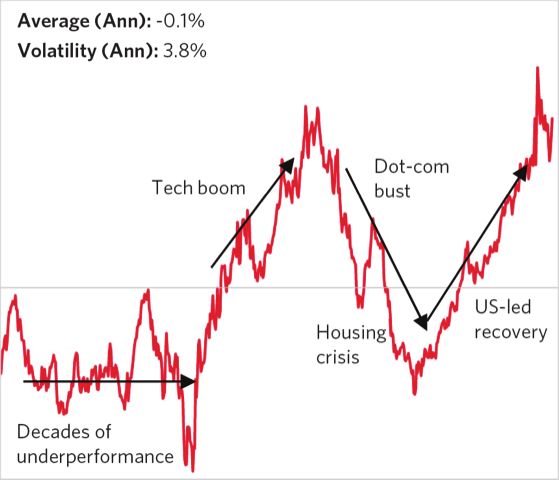
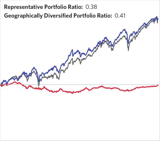
© 2020 Bridgewater Associates, LP 25Even so, while short-term correlations have been high, longer-term differences have big, compounded effects.
The charts below compare a representative US institutional investor portfolio (gray line) against a simple,
more geographically balanced version of the same portfolio (blue line); for example, we swap a US-heavy
equity allocation for an equal-weighted global equity mix, keeping equities’ overall share of the portfolio the
same. The difference between these two portfolios roughly isolates the uncompensated geographic risk in the
portfolio, shown in the red line below. It is striking that since 1960, a period over which the US has been the
single best equity market in the world, it still didn’t consistently pay to be geographically concentrated in the
US. A US-heavy portfolio slightly underperformed its more geographically balanced counterpart. The benefits
have been even bigger from the perspective of other equity markets and will be bigger in the future than they
have been in the recent past.
USA Representative Portfolio More Georgraphically Balanced Difference
Cumulative Excess Returns (ln, Hedged) 10yr Rolling Difference in Excess Returns
300% 60%
Representative Portfolio Ratio: 0.38 Average (Ann): -0.1%
Geographically Diversified Portfolio Ratio: 0.41 Volatility (Ann): 3.8%
200% 40%
Dot-com
100% Tech boom bust 20%
0% 0%
US-led
Housing recovery
crisis
-100% -20%
Decades of
underperformance
-200% -40%
1960 1970 1980 1990 2000 2010 2020 1970 1980 1990 2000 2010 2020 4
While the purpose of this three-part series is to work through the implications of a zero bond yield, and what
might be done about it, it is important to recognize that the problem does not exist in China, a huge and under-
invested market for most global investors. The 10-year bond yield in China is near 3% and in this turbulent
period has varied by enough that a) it was able to cushion some of the decline in the Chinese economy and
Chinese equities and b) it provided sufficient balance against the declines in other assets. So another path to
addressing the zero bond yield problem is to go where the problem does not exist.
4
Past results are not necessarily indicative of future results. Returns for the representative and more geographically balanced portfolios are simulated. Please review the Important
Disclosures located at the end of this research paper.
© 2020 Bridgewater Associates, LP 26USA Representative Portfolio Disclosure
The table below contains the allocation information for the historical simulation of the USA Representative Portfolio, from 1960 onwards, as well as
forward looking assumptions for expected ratio, volatility, and tracking error, used in this analysis. Correlations are based on either historical market
returns when available or Bridgewater Associates’ estimates, based on other available data and our fundamental understanding of asset classes.
The portfolio capital allocation weights (illustrated below) are estimates based either upon Bridgewater Associates’ understanding of standard
asset allocation (which may change without notice) or information provided by or publicly available from the recipient of this presentation. Asset
class returns are actual market returns where available and otherwise a proxy index constructed based on Bridgewater Associates understanding
of global financial markets. Information regarding specific indices and simulation methods used for proxies is available upon request (except
where the proprietary nature of information precludes its dissemination). Results are hypothetical or simulated and gross of fees unless otherwise
indicated. HYPOTHETICAL PERFORMANCE RESULTS HAVE MANY INHERENT LIMITATIONS, SOME OF WHICH ARE DESCRIBED BELOW. NO
REPRESENTATION IS BEING MADE THAT ANY ACCOUNT WILL OR IS LIKELY TO ACHIEVE PROFITS OR LOSSES SIMILAR TO THOSE SHOWN.
IN FACT, THERE ARE FREQUENTLY SHARP DIFFERENCES BETWEEN HYPOTHETICAL PERFORMANCE RESULTS AND THE ACTUAL RESULTS
SUBSEQUENTLY ACHIEVED BY ANY PARTICULAR TRADING PROGRAM. ONE OF THE LIMITATIONS OF HYPOTHETICAL PERFORMANCE
RESULTS IS THAT THEY ARE GENERALLY PREPARED WITH THE BENEFIT OF HINDSIGHT. IN ADDITION, HYPOTHETICAL TRADING DOES NOT
INVOLVE FINANCIAL RISK, AND NO HYPOTHETICAL TRADING RECORD CAN COMPLETELY ACCOUNT FOR THE IMPACT OF FINANCIAL RISK
IN ACTUAL TRADING. FOR EXAMPLE, THE ABILITY TO WITHSTAND LOSSES OR TO ADHERE TO A PARTICULAR TRADING PROGRAM IN SPITE
OF TRADING LOSSES ARE MATERIAL POINTS WHICH CAN ALSO ADVERSELY AFFECT ACTUAL TRADING RESULTS. THERE ARE NUMEROUS
OTHER FACTORS RELATED TO THE MARKETS IN GENERAL OR TO THE IMPLEMENTATION OF ANY SPECIFIC TRADING PROGRAM WHICH
CANNOT BE FULLY ACCOUNTED FOR IN THE PREPARATION OF HYPOTHETICAL PERFORMANCE RESULTS AND ALL OF WHICH CAN
ADVERSELY AFFECT ACTUAL TRADING RESULTS.
Asset Type Asset Nominal % Hedged Beta Beta Ratio Alpha Alpha Ratio
Exposure Fx Volatility Volatility
Equities Developed World Ex US Equities 19.0% 0% 14.9% 0.29 — —
Equities United States Equities 15.0% 0% 16.2% 0.25 — —
Equities United States Equities 15.0% 0% 16.2% 0.25 5.00% 0.25
Equities United States PE 9.0% 0% 26.7% 0.25 10.00% 0.25
MBS United States MBS 6.0% 0% 3.9% 0.25 — —
Corporate Bonds United States Corporate Bonds 5.0% 0% 7.3% 0.30 — —
Nominal Government Bonds United States Govt Bonds 5.0% 0% 4.8% 0.25 — —
Absolute Return Absolute Return 5.0% 0% — — 7.00% 0.50
Real Estate United States Real Estate 5.0% 0% 19.9% 0.25 6.00% 0.25
Nominal Government Bonds United States Govt Bonds 5.0% 0% 4.8% 0.25 2.00% 0.25
Equities Emerging Market Equities 3.0% 0% 21.1% 0.25 5.00% 0.30
High Yield Bonds United States High Yield Bonds 2.0% 0% 11.4% 0.30 — —
Nominal Government Bonds Developed World Bonds 2.0% 0% 4.1% 0.31 2.00% 0.30
Real Estate Developed World Real Estate 2.0% 0% 18.0% 0.31 6.0% 0.30
IL Bonds United States IL Bonds 1.0% 0% 6.0% 0.25 — —
IL Bonds United States IL Bonds 1.0% 0% 6.0% 0.25 1.00% 0.25
More Geographically Balanced Portfolio Disclosure
The “More Geographically Balanced” version of the portfolio preserves the portfolio’s asset class composition, but within each asset class distributes
capital equally across the following regions:
• Public Equities: USA, EUR, JPN, GBR, AUS, CAN, and EM
• Private Equities: USA, DEU, JPN, GBR, AUS, and CAN
• Nominal Government Bonds: USA, EUR, JPN, GBR, AUS, and CAN
• Inflation-Linked Bonds: USA, EUR, JPN, GBR, AUS, and CAN
• Corporate Bonds: USA, DEU, JPN, GBR, and AUS
For other asset classes, where data on the performance of individual regions’ assets are unavailable, the “More Geographically Balanced” version of
each portfolio retains that portfolio’s asset allocation. These asset classes include High-Yield Bonds, MBS, and Infrastructure. Results are hypothetical
or simulated and gross of fees unless otherwise indicated. Past results are not necessarily indicative of future results.
© 2020 Bridgewater Associates, LP 27You can also read