Guidance Trajectory Mathematical Modeling
←
→
Page content transcription
If your browser does not render page correctly, please read the page content below
Guidance Trajectory Mathematical Modeling
                                                                                                                            ∗†
                                                                                    Reza Rezaie and X. Rong Li

                                                                                            September 7, 2021

                                                                                                   Abstract
                                                    A trajectory of a destination-directed moving object (e.g. an aircraft from an origin airport to a destination
                                                airport) has three main components: an origin, a destination, and motion in between. We call such a trajectory
arXiv:2109.02141v1 [eess.SY] 5 Sep 2021

                                                that end up at the destination destination-directed trajectory (DDT). A class of conditionally Markov (CM)
                                                sequences (called CML ) has the following main components: a joint density of two endpoints and a Markov-
                                                like evolution law. A CML dynamic model can describe the evolution of a DDT but not of a guided object
                                                chasing a moving guide. The trajectory of a guided object is called a guided trajectory (GT). Inspired by
                                                a CML model, this paper proposes a model for a GT with a moving guide. The proposed model reduces
                                                to a CML model if the guide is not moving. We also study filtering and trajectory prediction based on the
                                                proposed model. Simulation results are presented.

                                            Keywords: Conditionally Markov sequence, dynamic model, destination-directed trajectory, guided trajec-
                                          tory, moving guide, filtering, prediction.

                                          1     Introduction
                                          Consider the problem of trajectory modeling with destination information, e.g., a flight from an origin to a
                                          destination. Such a problem has three main components: an origin, a destination, and motion in between. A
                                          Markov process, which can be described by an evolution law and an initial density, does not fit DDTs because
                                          it does not take the destination information into account in general. The CML sequence [1] has three main
                                          components: a joint endpoint density (in other words, an origin density and a destination density conditioned
                                          on the origin) and a Markov-like evolution law. CML sequences naturally fits the main DDT components [2].
                                          However, they cannot model GT with a moving guide.
                                            Trajectory modeling and trajectory prediction with an intent or a destination have been studied in the litera-
                                          ture. Some papers use a combination of the existing trajectory models without a destination and some heuristic
                                          modifications to handle trajectory modeling and prediction with destination information. These papers use esti-
                                          mation approaches developed for the case of no intent or destination and utilize intent/destination information
                                          to improve trajectory prediction [3]–[8]. In [3]–[5] the authors presented some trajectory prediction approaches
                                          based on hybrid estimation aided by intent information for air traffic control (ATC). In [6], the authors used a
                                          pseudo measurement approach to incorporate destination information and improve estimation results. In [7]–[8],
                                          a correlation factor and ADSB intent information was utilized to improve trajectory filtering and prediction in
                                          ATC. The above approaches are mainly based on a Markov model aided by some heuristic modifications due to
                                          the destination. But such models are not mathematically solid and hard to analyze. To study, generate, and
                                          analyze trajectories, it is desired to have a good mathematical model of trajectories providing a solid foundation
                                          for further studies.
                                             In some papers on trajectory modeling and prediction, trajectories are explicitly modeled without using heuris-
                                          tics. Due to uncertainty, trajectories are mathematically modeled by stochastic processes. Consider stochastic
                                          sequences defined over the time interval [0, N ] = (0, 1, . . . , N ). A sequence is Markov if and only if (iff) condi-
                                          tioned on the state at any time j, the segment before j is independent of the segment after j. A sequence is
                                          reciprocal iff conditioned on the states at any two times j and l, the segment inside the interval (j, l) is indepen-
                                          dent of the segments outside [j, l]. In other words, inside and outside [j, l] are independent given the boundaries.
                                          A sequence is CML iff conditioned on the state at time N , the sequence is Markov over [0, N − 1] [1]. Every
                                          Markov sequence is a reciprocal sequence (RS) and every RS is a CML sequence.
                                            ∗ The authors are with the Department of Electrical Engineering, University of New Orleans, New Orleans, LA 70148. Email

                                          addresses are rrezaie@uno.edu and xli@uno.edu.
                                             † Research supported by NASA through grant NNX13AD29A.

                                                                                                        1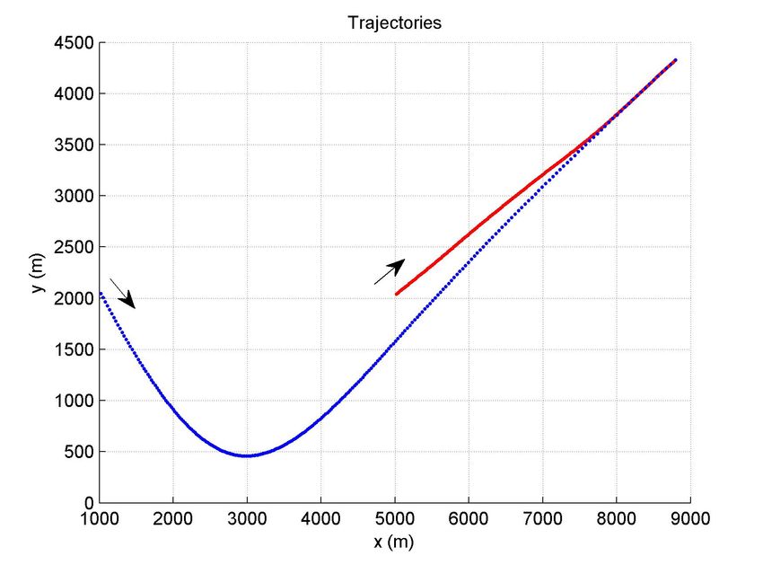
In [9] the problem of incorporating predictive information in a Markov model was considered. In [10]–[11], the
authors presented an approach for intent inference based on bridging distributions. That approach can be seen in
a reciprocal process (RP) setting, although RPs were not explicitly used or mentioned in [10]–[11]. Considering
quantized state space, [12]–[13] used finite-state RSs in intent inference and tracking. RPs are interesting for
modeling trajectories with a destination. But it is not always feasible or easy to quantize the state space. So,
it is desired to model trajectories as continuous-state, such as Gaussian sequences. In [14], a dynamic model
of nonsingular Gaussian (NG) RSs was presented. However, there are some difficulties about that model and
its extensions [15]. For example, due to the nearest-neighbor structure and dynamic noise correlation, state
estimation based on that model is not straightforward and several papers [16]–[20] were devoted to it. In [2], we
presented a model for DDTs using a CML model with white dynamic noise.
  GT modeling is important in many applications, including biology, robotics, aerospace, pursuit and evasion,
traffic control, and autonomous vehicles. Pursuit and evasion behavior, widely observed in nature, has a very
important role in predator foraging, prey survival, mating, and territorial battles in species [21]. In robotics,
pursuit and evasion games were used to study motion planning problems [22]. Trajectory of a vehicle pursuing
another one on a street is also a GT with a moving guide. GTs with a moving guide can also be found in a
problem with a team of unmanned aerial and ground vehicles pursuing another team of evaders [23]. Modeling
GTs with a moving guide is important in guidance, homing, and interception in aerospace applications [24]–[26].
An example is a moving object intercepting another moving object. A systematic approach for modeling a GT
with a moving guide in an appropriate mathematical model is desired.
  Gaussian CM processes were introduced in [27]. Inspired by [27], we presented definitions of different classes of
(Gaussian/non-Gaussian) CM processes (including CML ) in [1], where NG CM sequences were studied, modeled
and characterized [28]. Also, a dynamic model with white dynamic noise, called a CML model, was presented
for state evolution of NG CML sequences. As a special case of the CML model, a reciprocal CML model with
white noise was presented in [29]. In [30], we presented the notion of a Markov-induced CML model as a tool for
application of CML sequences.
   The main contributions of this paper are as follows. We propose a model to describe a GT with a moving
guide. The model is a generalization of our CML model for DDTs presented in [2]. We discuss parameter design
of the proposed model. Also, we derive trajectory filters and predictors based on the proposed trajectory model.
   The paper is organized as follows. In Section 2, a DDT modeling using CML sequences is reviewed. In Section
3, our proposed model for a GT with a moving guide is presented. Section 4 presents the corresponding trajectory
filter and predictor. Simulation examples are presented in Section 5. Section 6 contains conclusions.

2     DDT Modeling Using CML Sequences
The following notation is used:

                                               [i, j] , (i, i + 1, . . . , j − 1, j),       i
Without the notion of destination the trajectory of a moving object has two main elements: an origin and an
evolution law. A Markov sequence is determined by two elements: an initial density and an evolution law. Sample
paths of a Markov sequence can model such trajectories. A Markov sequence, with its final density uniquely
determined by its initial density and its evolution law, is not powerful or flexible enough for DDT modeling.

2.1    CML Sequences for DDT Modeling
Definition 2.3 ([1]) [xk ] is CML if

                                              F (ξk |[xi ]j0 , xN ) = F (ξk |xj , xN )                           (3)

∀j, k ∈ [0, N ], j < k, ∀ξk ∈ Rd .

  A CML model of the ZMNG CML sequence is as follows.

Theorem 2.4 ([1]) A ZMNG [xk ] is CML iff it obeys

                                     xk = Gk,k−1 xk−1 + Gk,N xN + ek ,             k ∈ [1, N − 1]                (4)

where [ek ] (Cov(ek ) = Gk ) is a ZMNG white sequence, and boundary condition

                                               x0 = e0 ,      xN = GN,0 x0 + eN                                  (5)

  Reciprocal sequences are special CML sequences.

Lemma 2.5 ([29]) [xk ] is reciprocal iff

                                              F (ξk |[xi ]j0 , [xi ]N
                                                                    l ) = F (ξk |xj , xl )                       (6)

∀j, k, l ∈ [0, N ] (j < k < l), ∀ξk ∈ Rd .

  Some desirable properties of CML sequences for DDT modeling are: 1) they model the main DDT components
well, 2) they have a Markov-like evolution law, which is simple and well understood, 3) the CML model can
systematically model the impact of destination on the evolution of trajectories, 4) the CML model has desirable
white dynamic noise, 5) state estimation based on the CML model is straightforward, and 6) CML sequences
(and their models) can be easily and systematically generalized, if necessary. However, the CML modeling of a
DDT assumes a fixed destination and cannot model trajectories with a moving destination.
   The structure of our CML model and that of the reciprocal model of [14] for DDT modeling are compared as
follows. The dynamic model presented in [14] has a nearest-neighbor structure, that is, the current state depends
on the previous state and the next state. So, information (density) of the next state is needed for estimation of
the current state, but such information is not available. Based on our CML model, information (density) about
the last state (destination) is required and available for DDT modeling in practice. In addition, the dynamic
noise in the model of [14] is colored, which makes state estimation not straightforward. By contrast, the dynamic
noise of our CML model is white and its state estimation is straightforward.
   For trajectory modeling we need nonzero-mean sequences. A nonzero-mean NG sequence is CML (or Markov)
iff its zero-mean part follows a CML model of Theorem 2.4 (or Lemma 2.2). A CML model of nonzero-mean
Gaussian CML sequences for DDT modeling is as follows. Let µ0 (µN ) and C0 (CN ) be the mean and covariance
of the origin (destination) state. Also, let C0,N be the cross-covariance of x0 and xN . We have (4) and

                                             xN = µN + GN,0 (x0 − µ0 ) + eN                                      (7)
                                              x0 = µ0 + e0                                                       (8)

where ek ∼ N (0, Gk ), k ∈ [0, N ], GN,0 = CN,0 C0−1 , GN = Cov(eN ) = CN − CN,0 C0−1 (CN,0 )0 , and G0 = C0 .

2.2    Parameter Design of CML Model for DDT
A DDT can be modeled based on two key assumptions [30]: (a) the motion follows a Markov model (2) (e.g.,
a nearly constant velocity model) without considering the destination information, and (b) the joint origin and
destination density is known (exactly or approximately). Now, let [sk ] be Markov modeled by (2). Since every
Markov sequence is CML , [sk ] can be modeled by a CML model (4) with (GsN = Cov(eN ), Gs0 = Cov(e0 ))

                                               s0 = e0 ,      sN = GsN,0 s0 + eN                                 (9)

                                                                   3
p(sk |sk−1 )p(sN |sk ,sk−1 )
where by p(sk |sk−1 , sN ) = p(sN |sk−1 ) = N (sk ; Gk,k−1 sk−1 + Gk,N sN , Gk ) and the Markov property,
∀k ∈ [1, N − 1], we have
Gk,k−1 = Mk,k−1 − Gk,N MN |k Mk,k−1 (10)
0 −1
Gk,N = Gk MN |k CN |k (11)
Gk = (Mk−1 + MN
0 −1
|k CN |k MN |k )
−1
(12)
where2 MN |N = I,
MN |k = MN,N −1 · · · Mk+1,k , k ∈ [1, N − 1]
N
X −1
0
CN |k = MN |n+1 Mn+1 MN |n+1 , k ∈ [1, N − 1]
n=k
and Mk,k−1 , Mk , k ∈ [1, N ], are parameters of (2).
Now, consider a different sequence [xk ] described by the same evolution model (4) but a different boundary
condition (5) with (Cov(eN ), GN,0 , Cov(e0 )) = (GN , GN,0 , G0 ) 6= (GsN , GsN,0 , Gs0 ). So, [sk ] and [xk ] are two
different sequences. By Theorem 2.4, [xk ] is a CML sequence. The sequences [sk ] and [xk ] have the same CML
evolution model/law (i.e., have the same parameters Gk,k−1 , Gk,N , Gk , k ∈ [1, N − 1]), but [xk ] can have any
joint endpoint density since parameters of its boundary condition (i.e., (GN , GN,0 , G0 )) are arbitrary.
The CML model (4) with parameters (10)–(12) is called the CML model induced by the Markov model (2) (or
simply the Markov-induced CML model) since its parameters are obtained from parameters of (2).
3 Modeling GT with a Moving Guide
A DDT can be naturally modeled as a CML sequence [xk ] as follows. The origin, the destination, and their
relationship are modeled by a joint density of x0 and xN . For a DDT, the density of xN is (assumed) known.
So, the evolution law is modeled as a density conditioned on xN . The simplest such density is the product of its
QN −1
−1
marginals: p([xk ]N
0 |x N ) = k=0 p(xk |xN ). But this conditionally independent law is often inadequate. Then,
N −1 QN −1
the next choice is often a CM density: p([xk ]0 |xN ) = p(x0 |xN ) k=1 p(xk |xk−1 , xN ), which is the evolution
law of a CML sequence. The main components of a CML sequence [xk ] are: a CM evolution law (conditioned on
xN ) and a joint density of x0 and xN . Similarly, we can consider more general and complicated evolution laws
(e.g., higher-order CM densities), if needed or desired. Therefore, by choosing conditional laws, a DDT can be
modeled well.
An illustrative application of GT with a moving guide is guidance, where object A (e.g., a missile) is chasing
(i.e., guided by) a moving object B (e.g., an aircraft). Object A is a guided object and object B is a moving
guide.
The above argument for DDTs does not work straightforwardly for a GT with a moving guide. It is explained
as follows. For a GT with a moving guide, the origin can be modeled similar to that of a DDT. However, since
the guide is moving (time varying), a random variable can not model it. Therefore, the motion of a moving guide
is modeled by a stochastic sequence. So, the whole problem, including the trajectory of the guided object and its
moving guide, can be modeled as follows. A GT is modeled by a sequence [xk ] and its moving guide trajectory
is modeled by a sequence [dk ]. Then, relationship between the two sequences should be determined. Following
this idea, a model is presented for a GT with a moving guide below.
Assume there is a moving object chasing a moving guide. The goal is to model the trajectory of the object
(i.e., GT) and its moving guide. Let the state evolution of the moving guide be modeled by a Markov sequence
[dk ]. So, we have
dk = Gdk,k−1 dk−1 + wk , k ∈ [1, N ], d0 = w0 (13)
where [wk ] is a white Gaussian sequence.
(13) can be any motion model (e.g., nearly constant velocity/acceleration/turn model).
A GT is modeled by a sequence [xk ] described by
xk = Gxk,k−1 xk−1 + Gxd
k,k−1 dk−1 + ek , k ∈ [1, N − 1] (14)
x0 = e0 (15)
xN = dN + eN (16)
2 By 0
matrix inversion lemma, (12) is equivalent to Gk = Mk − Mk MN 0
(CN |k + MN |k Mk MN )−1 MN |k Mk .
|k |k
4where [ek ] is a white Gaussian sequence uncorrelated with [wk ].
The above model for GT is justified as follows. At time k − 1 the object sets dk−1 as its guide. Then, following
the idea of DDT, the state evolution of the object at the moment is modeled by a CML model considering the
guide as its destination at the moment. The dynamic noise ek is used to model all stochastic deviations from the
deterministic relationship (i.e., (14) without ek ). The state evolution for the next time is justified in the same
way.
The underlying idea behind (14) is informally explained as follows. A random variable can model a time-
invariant phenomenon/effect. To describe a time-varying phenomenon/effect, a stochastic process is needed. To
model a GT with a moving guide, the final state of a CML sequence in its dynamic model is replaced by a
stochastic sequence that models the state evolution of the moving guide. Since the trajectory of the moving
guide is Markov in (13), the GT model (14) is called a Markov-guided CML -like model. It reduces to the model
(4) if the guiding sequence [dk ] reduces to the final state xN of the guided sequence (i.e., [dk ] = xN ).
It is well known how to determine parameters of the Markov model (13) of the moving guide, e.g., as a nearly
constant velocity/acceleration/turn model [31]. To determine parameters of (14), we follow the idea of a Markov-
induced CML model for a DDT: At any time we assume a moving guide to be fixed and treat the corresponding
dynamic model (14) as a DDT model. So, like the DDT model, parameters of (14) are determined for that time
based on the idea of a Markov-induced CML model. For simplicity, consider a time-invariant Markov model (2)
(e.g., a nearly constant velocity) with Mk,k−1 = F and Mk = Q. Then, by (10)–(12), the parameters of the
model (14) are determined as
Gk,k−1 = F − Gk,N F N −k+1 (17)
N −k 0 −1
Gk,N = Gk (F ) CN |k (18)
−1
Gk = (Q−1 + (F N −k )0 CN |k F
N −k −1
) (19)
PN −k−1
where CN |k = i=0 F i Q(F i )0 , k ∈ [1, N − 1].
Remark 3.1 (14) models a GT [xk ], where there is no destination for the moving guide (or information about
it). It is possible to extend model (14) to the case where the moving guide has its own destination, i.e., the
trajectory of the moving guide is destination-directed, resulting in a CML -guided CML -like model. Assume that
the moving guide sequence [dk ] has its own destination dN . Then, the trajectory of the object and its moving
guide are modeled as
xk = Gxk,k−1 xk−1 + Gxd
k,k−1 dk−1 + ek , k ∈ [1, N − 1] (20)
x0 = e0 (21)
xN = dN + eN (22)
dk = Gdk,k−1 dk−1 + Gdd
k,N dN + edk , k ∈ [1, N − 1] (23)
dN = Gdd d
N,0 d0 + eN (24)
d0 = ed0 (25)
where [ek ] and [edk ] are white Gaussian sequences, uncorrelated with each other.
In the above models, for simplicity, we assumed that the object reaches the guide at time N . However, it is
also possible to model trajectories where the object reaches the guide sooner than time N .
4 Trajectory Filtering and Prediction
Assume an object going towards its moving guide, where a sensor makes measurements of both the object and
its guide. The goal is to estimate the state of both the object and its guide. Since the object and its guide
are related, measurements for each one is useful for estimating the states of both. So, both states should be
estimated together using measurements of the object and its guide.
The measurements of the object and its guide are
zkx = Hk xk + vkx (26)
zkd = Hk dk + vkd (27)
where the measurement noise [vkx ]N d N
1 and [vk ]1 are zero-mean white, uncorrelated, and uncorrelated with [wk ] and
[ek ] of (13)–(14).
5Combining models (13) and (14), we have the Markov model
sk = Gk,k−1 sk−1 + esk (28)
zk = Hk sk + vk (29)
where
xk ek
sk = , esk = , Cov(esk ) = Gsk
dk wk
Gxk,k−1 Gxd
Gsk,k−1 = k,k−1
0 Gdk,k−1
Hkx
x x
0 zk vk
Hk = , zk = , vk =
0 Hkd zkd vkd
The goal is to obtain x̂k = E[xk |z k ] and dˆk = E[dk |z k ] and their mean square error (MSE) matrix given all the
measurements from the beginning to time k denoted as z k = {z1 , z2 , . . . , zk }. [esk ] and [vk ]N
1 are white Gaussian
sequences, uncorrelated with each other. By (28)–(29), sk and zk are linear combinations of [esk ] and [vk ]N 1 . So,
sk and zk are jointly Gaussian, and the minimum mean square error (MMSE) estimate of the states of the object
and its guide are
ŝk = E[sk |z k ] = ŝk|k−1 + Csk ,zk Cz−1
k
zk − H ŝ
k k|k−1 (30)
Σk = E[(sk − ŝk )(sk − ŝk )0 ] = Σk|k−1 − Csk ,zk Cz−1
k
(Csk ,zk )0 (31)
where
ŝk|k−1 = Gsk,k−1 ŝk−1
Σk|k−1 = Gsk,k−1 Σk−1 (Gsk,k−1 )0 + Gsk
Csk ,zk = Σk|k−1 (Hk )0
Czk = Hk Σk|k−1 (Hk )0 + Rk
and the estimate of xk and its MSE matrix are
x̂k = [I, 0]ŝk
Pkx = [I, 0]Σk [I, 0]0
and the estimate of dk and its MSE matrix are
dˆk = [0, I]ŝk
Pkd = [0, I]Σk [0, I]0
Trajectory is predicted as follows. Let [sk ] be modeled by (28). Assume that the output of the filter p(sk |z k ) =
N (sk ; ŝk , Σk ) at time k is available. For k + n ∈ [k + 1, N − 1], the prediction and its MSE matrix are obtained
as
ŝk+n|k = Gsk+n|k ŝk (32)
Σk+n|k = Ck+n|k + Gsk+n|k Σk (Gsk+n|k )0 (33)
where Gsk|k = I, ∀k, and
Gsk+n|k = Gsk+n,k+n−1 Gsk+n−1,k+n−2 · · · Gsk+1,k
k+n−1
X
Ck+n|k = Gsk+n|i+1 Gsi (Gsk+n|i+1 )0
i=k
Then, the prediction of xk+n and its MSE matrix are
x̂k+n|k = [I, 0]ŝk+n|k (34)
x 0
Pk+n|k = [I, 0]Σk+n|k [I, 0] (35)
6Figure 1: Trajectory of a guided object (blue line) chasing its moving guide (red line).
The prediction of dk+n and its MSE matrix are
dˆk+n|k = [0, I]ŝk+n|k (36)
d 0
Pk+n|k = [0, I]Σk+n|k [0, I] (37)
Filtering and prediction based on (20)–(23) are similar. Combining (20) and (23), we have the Markov model
sk = Gsk,k−1 sk−1 + esk (38)
zk = Hk sk + vk (39)
where
Gxk,k−1 Gxd
k,k−1 0
Gsk,k−1 = 0 Gdk,k−1 Gdd k,N
0 0 I
x
xk ek
sk = dk , esk = edk
dN 0
x
x x
Hk 0 0 zk vk
Hk = , zk = , vk =
0 Hkd 0 zkd vkd
Then, filtering and prediction are based on (38)–(39).
5 Simulations
A simulation study of the proposed model for modeling GT with a moving guide is reported in this section.
Assume a two-dimensional scenario, where the state of a moving object at time k is xk = [x, ẋ, y, ẏ]0k with
position [x, y]0 and velocity [ẋ, ẏ]0 . The state of the moving guide dk is defined similarly.
Let the GT of a moving object be modeled by (14) and the trajectory of its moving guide by (13). Parameters
of
d 1 T
the Markov model (13) are Gk,k−1 = diag(F1 , F1 ) and Cov(wk ) = diag(Q1 , Q1 ), k ∈ [1, N ], where F1 = ,
0 1
3
T /3 T 2 /2
Q1 = q , T = 1 second, q = 0.005, and N = 250. Also, parameters of (14) are given by (17)–(19),
T 2 /2 T
where F = diag(F1 , F1 ) and Q = diag(Q1 , Q1 ).
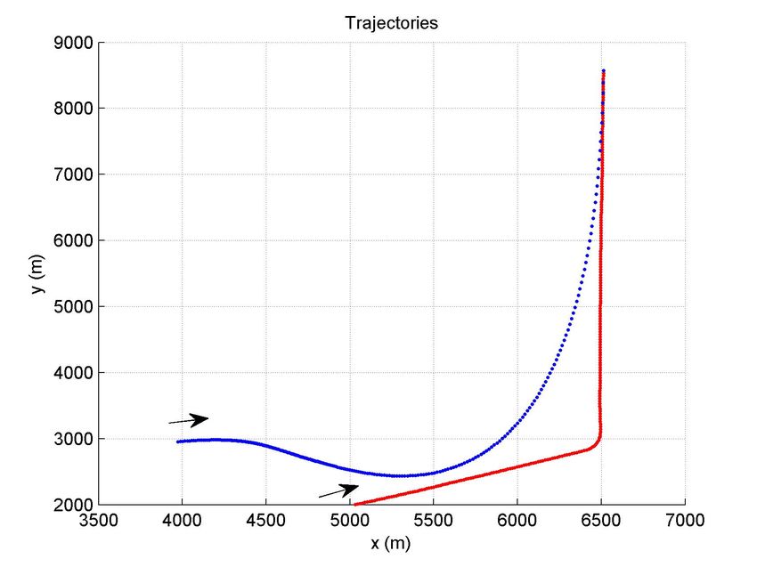
Figs. 1, 2, 3 show the GT of an object (blue line) along with that of its moving guide (red line) in three
scenarios. They show how the object can chase and reach its moving guide, where there are different initial
states of the object and its guide.
6 Conclusions
CML sequences model DDTs well, but they cannot model well a GT with a moving guide because they cannot
take a moving guide into account. This is because a CML sequence models the destination of a DDT by the final
7Figure 2: Trajectory of a guided object (blue line) chasing its moving guide (red line).
Figure 3: Trajectory of a guided object (blue line) chasing its moving guide (red line).
8state of the sequence. The final state is a random variable and does not change over time. A stochastic sequence
is needed to model the trajectory of a moving guide.
Inspired by a CML dynamic model, a model has been proposed for a GT with a moving guide. Model parameter
design and the corresponding optimal trajectory filtering and prediction have been also studied.
Following the idea of DDT modeling by a CML sequence, the proposed GT model has been extended to the
case where the moving guide has its own destination.
CM sequences/models are powerful modeling tools. For example, a CML dynamic model can describe a DDT
straightforwardly. Although a CML model cannot directly take a moving guide into account to model a GT, it
provides a foundation for a model that can describe GT with a moving guide.
References
[1] R. Rezaie and X. R. Li. Nonsingular Gaussian Conditionally Markov Sequences. IEEE West. New York Image
and Signal Processing Workshop, Rochester, NY, USA, pp. 1-5, Oct. 2018.
[2] R. Rezaie and X. R. Li. Destination-Directed Trajectory Modeling and Prediction Using Conditionally Markov
Sequences. IEEE West. New York Image and Signal Processing Workshop, Rochester, NY, USA, pp. 1-5, Oct.
2018.
[3] I. Hwang and C. E. Seah. Intent-Based Probabilistic Conflict Detection for the Next Generation Air Trans-
portation System. Proceedings of the IEEE, vol. 96, no 12, pp. 2040-2058, Dec. 2008.
[4] J. Yepes, I. Hwang, and M. Rotea. An Intent-Based Trajectory Prediction Algorithm for Air Traffic Control.
AIAA Guidance, Navigation, and Control Conf., San Francisco, CA, USA, pp.1-15, Aug. 2005.
[5] Y. Liu and X. R. Li. Intent-Based Trajectory Prediction by Multiple Model Prediction and Smoothing. AIAA
Guidance, Navigation, and Control Conf., Kissimmee, Florida, USA, pp. 1-15, Jan. 2015.
[6] G. Zhou, K. Li, X. Chen, L. Wu, and T. Kirubarajan. State Estimation with Destination Constraint Using
Pseudo-measurements. Signal Processing, vol. 145, pp. 155-166, Apr. 2018.
[7] J. Krozel and D. Andrisani. Intent Inference and Strategic Path Prediction. J. of Guidance, Control, and
Dynamics, vol. 29, no. 2, pp. 225-236, Mar-Apr. 2006.
[8] K. Mueller and J. Krozel. Aircraft ADS-B Intent Verification Based on Kalman Tracking Filter. AIAA Guid-
ance, Navigation, and Control Conf., Denver, CO, USA, pp. 1-15, Aug. 2000.
[9] D. A. Castanon, B. C. Levy, and A. S. Willsky. Algorithms for Incorporation of Predictive Information in
Surveillance Theory. Inter. J. of Systems Science, vol. 16, no. 3, pp. 367-382, 1985.
[10] B. I. Ahmad, J. K. Murphy, S. J. Godsill, P. M. Langdon, and R. Hardy. Intelligent Interactive Displays in
Vehicles with Intent Prediction: A Bayesian Framework. IEEE Signal Processing Magazine, vol. 34, no. 2,
pp. 82-94, Mar. 2017.
[11] B. I. Ahmad, J. K. Murphy, P. M. Langdon, and S. J. Godsill. Bayesian Intent Prediction in Object Tracking
Using Bridging Distributions. IEEE Trans. on Cybernetics. vol. 48, no. 1, pp. 215-227, Dec. 2018.
[12] M. Fanaswala and V. Krishnamurthy. Detection of Anomalous Trajectory Patterns in Target Tracking via
Stochastic Context-Free Grammar and Reciprocal Process Models. IEEE J. of Selected Topics in Signal
Processing, vol. 7, no. 1, pp. 76-90, Feb. 2013.
[13] M. Fanaswala, V. Krishnamurthy, and L. B. White. Destination-aware Target Tracking via Syntactic Signal
Processing. IEEE Inter. Conf. on Acoustics, Speech and SP (ICASSP), Prague, Czech, pp. 3692-3695, May
2011.
[14] B. C. Levy, R. Frezza, and A. J. Krener. Modeling and Estimation of Discrete-Time Gaussian Reciprocal
Processes. IEEE Trans. on Automatic Control, vol. 35, no. 9, pp. 1013-1023, Sep. 1990.
[15] L. B. White and F. Carravetta. Stochastic Realization and Optimal Smoothing for Gaussian Generalized
Reciprocal Processes. IEEE Conf. on Decision and Control, Melbourne, Australia, pp. 369-374, Dec. 2017.
[16] C. Greene and B. C. Levy. Some New Smoothers Implementations for Discrete-time Gaussian Reciprocal
Processes. Inter. J. of Control, vol. 54, no. 5, pp. 1233-1247, 1991.
9[17] E. Baccarelli and R. Cusani. Recursive Filtering and Smoothing for Gaussian Reciprocal Processes with
Dirichlet Boundary Conditions. IEEE Trans. on Signal Processing, vol. 46, no. 3, pp. 790-795, Mar. 1998.
[18] S. Bernstein. Sur Les Liaisons Entre Les Grandeurs Aleatoires. Verhand. Internat. Math. Kongr., Zurich,
(Band I), 1932.
[19] D. Vats and J. M. F. Moura. Recursive Filtering and Smoothing for Discrete-Index Gaussian Reciprocal
Processes. 43rd Annual Conf. on Information Sciences and Systems, Baltimore, MD, USA, pp. 377-382, Mar.
2009.
[20] D. Vats and J. M. F. Moura. Telescoping Recursive Representations and Estimation of Gauss–Markov
Random Fields. IEEE T-IT, vol. 57, no. 3, pp. 1645-1663, Mar. 2011.
[21] D. Pais and N. E. Leonard. Pursuit and Evasion: Evolutionary Dynamics and Collective Motion. AIAA
Guidance, and Control Conf., Toronto, ON., Canada, pp. 1-14, 2010.
[22] T. H. Chung, G. A. Hollinger, and V. Isler. Search and Pursuit-Evasion in Mobile Robotics. Autonomous
Robots, vol. 31, no. 299, July 2011.
[23] R. Vidal, O. Shakernia, H. J. Kim, David H. Shim, and S. Sastry. Probabilistic Pursuit-Evasion Game:
Theory, Implementation, and Experimental Evaluation. IEEE Trans. on Robotics and Automation, vol. 18,
no. 5, pp. 662-669, Dec. 2002.
[24] M. D. Ardema and N. Rajan. An Approach to Three-Dimensional Aircraft Pursuit-Evasion. Computers,
Mathematics with Applications, vol. 13, no. 1-3, pp. 97-110, 1987.
[25] M. Pachter and Y. Yavin. Simple-Motion Pursuit-Evasion Differential Games, Part 1: Stroboscopic Strategies
in Collision-Course Guidance and Proportional Navigation. J. of Optimization Theory and Applications, vol.
51, no. 1, pp. 95-127, Oct. 1986.
[26] M. Pachter and Y. Yavin. Simple-Motion Pursuit-Evasion Differential Games, Part 2: Optimal Evasion from
Proportional Navigation Guidance in the Deterministic and Stochastic Cases. J. of Optimization Theory and
Applications, vol. 51, no. 1, pp. 129-159, Oct. 1986.
[27] C. B. Mehr and J. A. McFadden. Certain Properties of Gaussian Processes and Their First-Passage Times.
J. of Royal Statistical Society, (B), vol. 27, pp. 505-522, 1965.
[28] R. Rezaie. Gaussian Conditionally Markov Sequences: Theory with Application. PhD Dissertation, University
of New Orleans, 2019.
[29] R. Rezaie and X. R. Li. Gaussian Reciprocal Sequences from the Viewpoint of Conditionally Markov Se-
quences. Inter. Conf. Vision, Image and Signal Processing, Las Vegas, NV, USA, pp. 33:1-33:6, Aug. 2018.
[30] R. Rezaie and X. R. Li. Gaussian Conditionally Markov Sequences: Dynamic Models and Representations
of Reciprocal and Other Classes. IEEE Trans. on Signal Processing, vol. 68, pp. 155-169, 2020.
[31] X. R. Li and V. P. Jilkov. Survey of Maneuvering Target Tracking Part I: Dynamic Models. IEEE Trans.
on Aerospace and Electronic Systems, vol. 39, no. 4, pp. 1333-1364, Oct. 2003.
[32] R. Rezaie and X. R. Li. Gaussian Conditionally Markov Sequences: Algebraically Equivalent Dynamic
Models. IEEE Trans. on Aerospace and Electronic Systems, vol. 56, no. 3, pp. 2390-2405, 2020.
[33] R. Rezaie and X. R. Li. Gaussian Conditionally Markov Sequences: Modeling and Characterization. Auto-
matica, vol. 131, 2021.
[34] R. Rezaie and X. R. Li. Gaussian Conditionally Markov Sequences: Singular/Nonsingular. IEEE Trans. on
Automatic Control, vol. 65, no. 5, pp. 2286-2293, 2020.
[35] R. Rezaie and X. R. Li. Trajectory Modeling and Prediction with Waypoint Information Using a Condition-
ally Markov Sequence. In 2018 56th Annual Allerton Conference on Communication, Control, and Computing
(Allerton), Monticello, IL, USA, pp. 486-493, Oct. 2018.
[36] R. Rezaie and X. R. Li. Destination-Directed Trajectory Modeling, Filtering, and Prediction Using Condi-
tionally Markov Sequences. IEEE Trans. on Aerospace and Electronic Systems, vol. 57, no. 2, pp. 820-833,
2020.
[37] R. Rezaie and X. R. Li. Conditionally Markov Modeling and Optimal Estimation for Trajectory with Way-
points and Destination. IEEE Trans. on Aerospace and Electronic Systems, vol. 57, no. 4, pp. 2006-2020,
2021.
10[38] R. Rezaie and X. R. Li. Models and Representations of Gaussian Reciprocal and Conditionally Markov
Sequences. Inter. Conf. Vision, Image and SP, Las Vegas, NV, USA, pp. 66:1-66:6, Aug. 2018.
11You can also read