Hanbury Brown-Twiss correlations and multi-mode dynamics in quenched, inhomogeneous density spinor Bose-Einstein condensates - IOPscience
←
→
Page content transcription
If your browser does not render page correctly, please read the page content below
PAPER • OPEN ACCESS

Hanbury Brown–Twiss correlations and multi-mode dynamics in
quenched, inhomogeneous density spinor Bose–Einstein condensates
To cite this article: A Vinit and C Raman 2018 New J. Phys. 20 095003

View the article online for updates and enhancements.

                              This content was downloaded from IP address 46.4.80.155 on 25/12/2020 at 16:11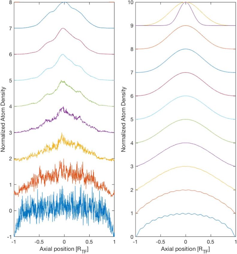
New J. Phys. 20 (2018) 095003 https://doi.org/10.1088/1367-2630/aadc74
PAPER
Hanbury Brown–Twiss correlations and multi-mode dynamics in
OPEN ACCESS
quenched, inhomogeneous density spinor Bose–Einstein
RECEIVED
22 December 2017 condensates
REVISED
11 July 2018
A Vinit and C Raman
ACCEPTED FOR PUBLICATION
23 August 2018
School of Physics, Georgia Institute of Technology, Atlanta, Georgia 30332, United States of America
PUBLISHED
E-mail: chandra.raman@physics.gatech.edu
12 September 2018
Keywords: spinor condensate, non-equilibrium, Hanbury Brown–Twiss, quantum quench, quantum phase transition
Original content from this
work may be used under
the terms of the Creative Abstract
Commons Attribution 3.0
licence. We have studied the effects of multiple, competing spatial modes that are excited by a quantum
Any further distribution of quench of an antiferromagnetic spinor Bose–Einstein condensate. We observed Hanbury Brown–
this work must maintain
attribution to the Twiss correlations and associated super-Poissonian noise in the mode populations. The decay of these
author(s) and the title of
the work, journal citation
correlations was consistent with experimentally observed spin domain patterns. Data were compared
and DOI. with a real-space Bogoliubov theory as well as numerical solution of the coupled Gross–Pitaevskii
equations that were seeded by quantum noise via the truncated Wigner approximation. The spatial
modes that were both observed experimentally and deduced theoretically are intimately connected to
the inhomogeneous density profile of the condensate. Unique features were observed not present in a
homogeneous system, including unstable modes located near the center of the cloud, where the
dynamics were initiated.
1. Introduction
Quantum phase transitions have become an important arena of exploration using ultracold atoms. In contrast to
the traditional view of these transitions that has focused on equilibrium properties [1], quantum gases afford a
dynamical view made experimentally possible by rapidly quenching the system [2]. A major advantage exists for
such quench experiments over equilibrium studies very close to the critical point, where the timescales become
longer and the equilibration condition harder to fulfill. Instead, in a quench scenario, the transition is crossed
very rapidly from well outside its boundaries. If the system has no time to respond to the change, then a full
panoply of dynamical behavior can be observed that is characteristic of the symmetries broken by the transition
(see figure 1). This includes (i) instability of the initial state and formation of seeds of the ground state on the
opposite side of the critical point, (ii) rapid expansion of the seeds to macroscopic proportions, with damped
oscillations due to the finite system size, and (iii) slow growth to steady-state. Using this approach, we have
recently been able to make sub-Hz level (picoKelvin) precision measurements on the transition boundary in an
antiferromagnetic spinor Bose–Einstein condensate, although the system temperature was 400 nK [3], well
above the energy scales of the phase transition itself.
In the present work we extend our earlier studies on the q=0 quantum phase transition in
antiferromagnetic spinor Bose–Einstein condensates (BECs). We present measurements of Hanbury Brown and
Twiss correlations and study their decay length. While our previous works have confirmed the Bogoliubov
predictions for the instability rate [3, 5], here we provide many details—both experimental and theoretical—
that were missing in the earlier works. For instance, we use statistical analysis to elucidate the variety and wealth
of modes that were observed to form in the experiment, and compare with Bogoliubov predictions for these
modes. Similar to the quench experiments of [6], we have observed that the maximally unstable modes are
localized near the center of the cloud, where the density is highest. We show that this result appears naturally
from the real space calculation of the Bogoliubov eigenvectors, which are different from the momentum modes
typical of a homogeneous BEC.
© 2018 The Author(s). Published by IOP Publishing Ltd on behalf of Deutsche Physikalische Gesellschaft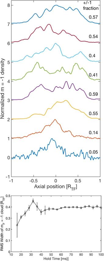
New J. Phys. 20 (2018) 095003 A Vinit and C Raman
Figure 1. Quantum quenches reveal two phases of an antiferromagnetic spinor BEC. (a) Quantum phase transition between polar and
antiferromagnetic (AF) phases at zero quadratic Zeeman shift q. (b) Dynamical instability induced by a rapid quench from q1>0 to
q20 or ferromagnetic for c20. The overall density profile n(r) is determined by the chemical potential μ, which is larger in magnitude
by a factor of 100 compared with equation (1) for typical values of q. Thus, we have removed the spin-
independent terms from the Hamiltonian, which are assumed to be a constant. Fˆ, Fˆz are the vector spin-1
operator and its z-projection, respectively. Hereafter in this work, we write m≡mF.
The second term in equation (1) is the quadratic Zeeman shift due to the external magnetic field,
q = qB˜ 02 + qM . B0 is the magnetic field at the trap center, q̃ = 276 Hz Gauss−2 is the coefficient of the quadratic
Zeeman shift for sodium atoms, and gF = 1 2 and μB are the Lande g-factor and Bohr magneton, respectively
[17]. In addition to the static magnetic field, we introduce an additional term qM, which is the shift caused by a
microwave magnetic field through the AC Zeeman effect on the F=1, m sublevels [4, 5]. The microwave field
generates an additional shift qM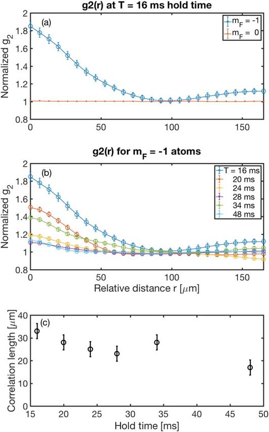
New J. Phys. 20 (2018) 095003 A Vinit and C Raman
superposition of two components m=±1, a so-called antiferromagnetic phase [18]. We study the effect of a
quantum quench across the zero temperature quantum phase transition at q=0.
2.2. Experimental method
Sodium Bose–Einstein condensates in a single focus optical trap were prepared in the m=0 state in a static
magnetic field. The protocol is described in earlier work [5], but we include relevant details here. The peak
density n0=5×1014 cm−3 and axial Thomas–Fermi radius Rx=340 μm were measured to an accuracy of
5%, from which we determined the peak spin-dependent interaction energy c2n0=h×120 Hz. The axial and
radial trapping frequencies were 7 and 470 Hz, respectively, accurate to 10%. The radial Thomas–Fermi radius
was R^ = 5 μm, and thus the aspect ratio of the cigar-shaped cloud was ≈70:1. The measured temperature was
400 nK, close to the chemical potential of 360 nK.
Our experiment required precise control over the bias magnetic field. We applied a magnetic field Bx aligned
with the long axis x of the cigar and tuned the field gradient dBx /dx to cancel ambient field inhomogeneities in
our vacuum chamber to within±10 μG over the sample using a procedure that is described in [3]. The
microwave field used to control qM was generated by an HP8648B synthesizer with∼100 Hz accuracy. Its
frequency was tuned below the ‘clock’ transition, ∣F = 1, m = 0ñ ∣F = 2, m = 0ñ at 1.772 GHz [19] by an
amount between 260 and 470 kHz, resulting in a negative shift qM0 to a final value qf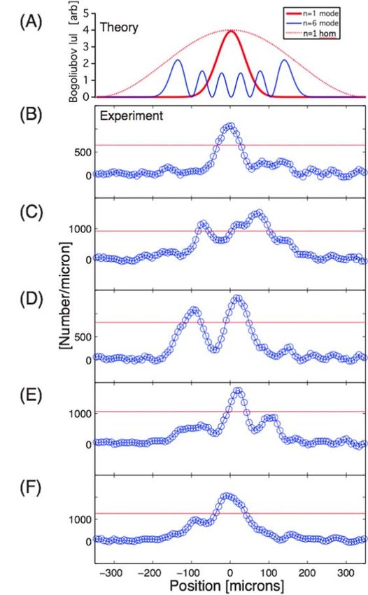
New J. Phys. 20 (2018) 095003 A Vinit and C Raman
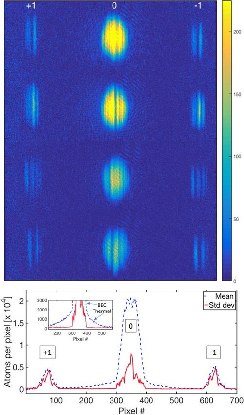
Figure 2. Stochastic nature of the quench. Upper panel shows time-of-flight Stern–Gerlach images of 4 distinct, but otherwise
identically prepared quenched Bose–Einstein condensates after a hold time of 20 ms. Each image is 1.3 × 4.6 mm in size. Lower panel
shows mean and standard deviation of one-dimensional slices through the images. The inset is a blow-up of the m = 0 condensate.
fluctuation is not due to technical reasons, but is a fundamental feature of the quench, as unoccupied spin
excitation modes become rapidly occupied, with a highly variable number and mode distribution.
We analyzed these fluctuations using statistical methods on an ensemble of measurements on identically
prepared BECs. Thirty images were collected at each quench hold time, whose mean atom number N̄ and
standard deviation σN were computed. We suppressed shot to shot atom number fluctuations by filtering only
those whose atom number lay inside the range N¯ < N < N¯ + sN , resulting in samples with less than 10%
atom number fluctuations. This allowed us to more clearly observe the intrinsic noise.
For this filtered data set, each camera image was reduced to a one-dimensional slice f (x), where x is the axial
coordinate within the image. To accomplish this, we converted the absorption images to atomic column density
(atoms/pixel2) through the known absorption cross-section for light resonant with the F = 2 F ¢ = 3
transition [22, 23]. We then summed each image over the central 75% of the time-of-flight Thomas–Fermi
distribution along the radial direction. The domain of the sum was chosen to maximize the number of atoms
counted without introducing excess noise from the edges of the Thomas–Fermi distribution where the atom
numbers were smaller than image noise. The resulting set of slices f (x), calibrated in atoms/pixel, were
processed to derive mean and standard deviations. The lower panel of figure 2 shows these as dashed blue and
solid red lines, respectively. It is clearly visible in the figure that the m=0 number density fluctuations were no
more than 40% of the mean, while those of the m=±1 cloud were as much as 100% of the mean. As we will
show, the two noise sources in fact have the same origin.
These results are intriguing, since a Bose–Einstein condensate is not expected to have 100% variability in
atom number. Similar to laser light, a BEC can be described by a coherent state, with Poissonian number density
4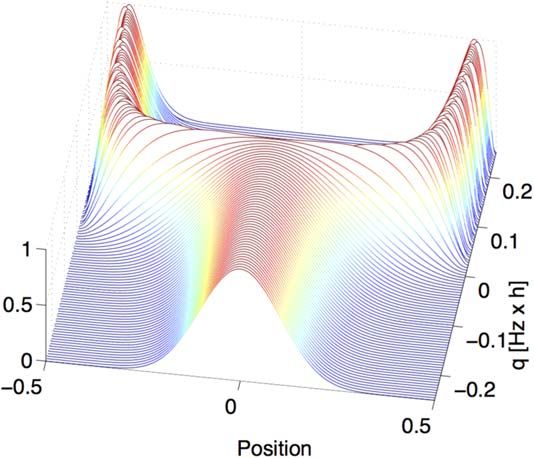
New J. Phys. 20 (2018) 095003 A Vinit and C Raman
fluctuations (shot noise). In the absence of any quench, an analysis of individual pixels showed that the m=0
cloud possessed a variance quite close to this limit. For shot noise, the ratio of standard deviation to mean atom
number density áDnñ n¯ = 1 n¯ is very small for the large atom numbers present in the experiment. By
contrast, the m=±1 clouds show ‘super-Poissonian’ (SP) noise with áDnñ n¯ = 1. We note that SP
fluctuations have been observed in related works where spin-exchange collisions are responsible for the
statistical fluctuations [24, 25].
3.2. Role of thermal atoms in the quench
Our data in the inset to the lower panel of figure 2 also reveal that thermal atoms play a negligible role in the
quench. The m=0 cloud can be seen to possess a bimodal distribution in space, with the central, sharp peak
corresponding to the Bose–Einstein condensate and a lower density, more diffuse pedestal due to the thermal
atoms whose occupation fraction was 40%, corresponding to a temperature of T∼400 nK.
In spite of such a large thermal population, at short hold times the fluctuations (the red curve in the inset)
drop sharply to zero at the Thomas–Fermi radius. Therefore the spin dynamics clearly occur only in the
condensate, and not in the normal gas. At longer hold times t=48 ms (not shown in the figure), the m=±1
populations had grown substantially to comprise a fraction 0.6 of the total condensate. By this time, a thermal
gas of m=±1 atoms had become populated via interactions between the thermal cloud in m=0 and various
condensed spin components [26]. Nonetheless, the m=−1 spin fluctuations (and therefore, spin relaxation
dynamics) still continued to occur only in the condensate, and not in the normal gas.
Our results can be summarized as coherent spin evolution for short times, followed by thermally assisted
spin redistribution occurring at long hold times. The separation of timescales poses the intriguing possibility to
cool the sample via spin-changing collisions and selective spin state removal of the thermal cloud.
3.3. Hanbury Brown–Twiss correlations
Turning now to the condensed components, the super-Poissonian fluctuations mentioned earlier lead to
Hanbury Brown–Twiss correlations in our spatially extended one-dimensional system. Such correlations have
been widely observed from the domain of radio-frequencies where they were initially observed and used to
determine the angular diameter of stars [27] to the optical domain [28]. For massive particles, these correlations
have been observed with ensembles of ultracold atoms [29–31], as well as in the sub-atomic realm, where one
can use them to extract information about nuclear structure from collisions [32]. In our experiment with
Bose–Einstein condensates they reveal the coherence length associated with the non-equilibrium state created
by the quench.
We examined the second order spin density correlation function g2(x) with relative coordinate x between
points of observation:
á n ( x 0 + x ) n ( x 0) ñ
g2 (x ) = . (2)
án (x 0 + x )ñán (x 0)ñ x0
Here n(x0) is the density of a particular spin component, for example, the m=−1 atoms, and x0 represents a
spatial position within the cloud. The inner and outer brackets refer to ensemble and spatial averages,
respectively. Since the Thomas–Fermi density profile breaks translation invariance in the system, we define
ensemble and spatial averages to be distinct quantities. First ensemble averages were taken over a restricted set of
images with reduced atom number fluctuations as discussed earlier, after which a spatially averaged g2 was
computed over all values of x0. For each data set we performed bimodal fits to the central, m=0 cloud to
determine the condensate Thomas–Fermi radius RTF. From the mean of the m=±1 slices we computed the
central position xc of the m=±1 clouds in order to undo the Stern–Gerlach expansion. From xc and RTF we
could generate distributions n−1(x) within the cloud. Since one divides by the mean value to compute g2, its value
blows up as one approaches the distribution edges—to avoid this, we restricted our analysis to
−RTF/2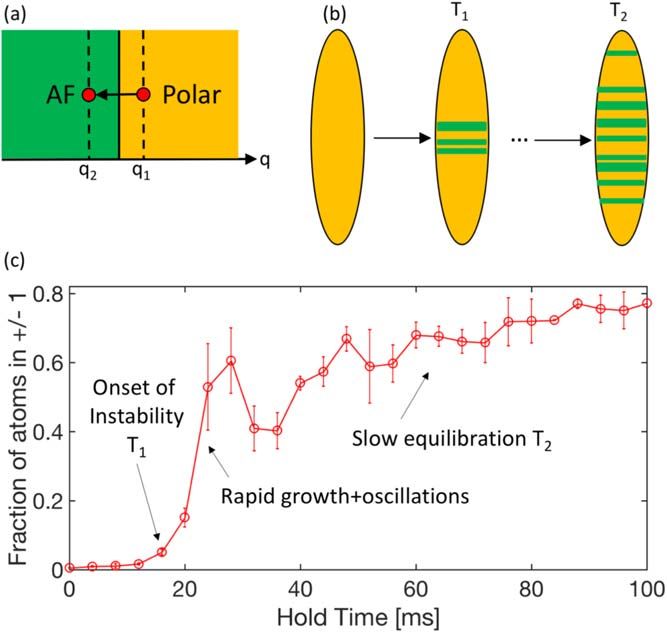
New J. Phys. 20 (2018) 095003 A Vinit and C Raman
Figure 3. Hanbury Brown–Twiss correlations. (a) and (b) Second order correlation functions g2(x) versus separation x, for parameters
defined in the text. Error bars are statistical. (c) Correlation length defined as the half-width of g2−1. Error bars are the experimental
resolution.
Corresponding data for m=+1 was similar to −1. The data clearly show a very strong ‘spin bunching’ effect, as
individual m=−1 atomic spins tend to be co-located, with g2(0)=1.9>1. This was observed very early in the
quench, when the m=±1 atom numbers were very small, and the corresponding fluctuations proportionally
large. The measured value of g2(0) close to 2 is consistent with a thermal state and the super-Poissonian noise in
the population.
In contrast to the above bunching phenomenon, the m=0 spins exhibited very little bunching—the
measured g2(x) was very close to 1 for all values of x, consistent with a Bose–Einstein condensate in a coherent
state. Upon closer examination, we determined that g2(0) – 1≈0.01. This small excess in the normalized
variance can be largely explained by technical noise caused by atom number fluctuations as well as spin-
exchange noise in the mF=0 population due to the production of m=±1. The former (latter) had a standard
deviation of 7% (5%), and were thus of the same magnitude at this early hold time. For only slightly later times of
t 20 ms, the stochastic fluctuations of the quench became 40% as noted earlier in figure 2, and dominated
over technical noise.
For the m=−1 atoms, figure 3(b) shows that g2(x) rapidly decays in space, exhibiting damped oscillations
g (x ) - 1
that approach a value of 1. Defining the correlation length, x1/2, through the formula 2g (10)2 - 1 = 0.5 we
2
obtained x1/2=33 μm. This correlation length is substantially smaller than the condensate Thomas–Fermi
radius RTF=340 μm, and reveals the average spatial extent of the spin modes excited by the quench. The
oscillations in the g2 function indicated the formation of multiple domains simultaneously, and is further
evidence of the multi-mode character that we explore in the next section. Individual images revealed domains
between 15 and 45 μm in size (see figure 6). The middle panel of figure 3 shows that for slightly longer hold times
where the ratio of m=±1 to m=0 populations became appreciable, g2 (0) 1 indicating the formation of a
6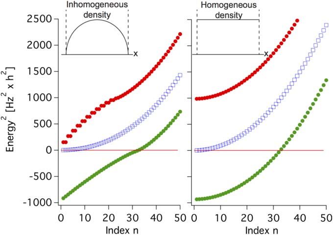
New J. Phys. 20 (2018) 095003 A Vinit and C Raman
Figure 4. Quantum spin thermalization. Shown are the probability distributions for m = -1 atoms at a hold time of 20 ms, at
different spatial locations x0 within the cloud that have varying mean atom number n¯ (x 0 ). Each graph uses 20 bins covering the region
of non-zero data, approximately 0 < n < 3n¯ (x 0 ) . Good agreement is found with the Bose–Einstein distribution (equation (3), solid
curves) which uses the local sample average n¯ (x 0 ) but otherwise has no fitting parameters.
more stable, non-equilibrium state. In spite of this, the population in ±1 had not yet reached its equilibrium
value. The lower panel of figure 3 shows that the correlation length shrinks by a factor of about 2 with hold time
(although an oscillation in the population seen in figure 1 causes it to momentarily increase at 34 ms). Thus the
system transferred energy from long to short wavelength modes as the quench progressed.
3.4. Boltzmann statistics for the spin
How does a thermal state appear within a Bose–Einstein condensate, whose dynamics are governed by quantum
mechanics? A closely related, and more general question is how isolated quantum systems thermalize when
placed out of equilibrium [2]. One answer that has emerged in recent years addresses the similarity between
quantum and thermal fluctuations, particularly when one looks at the system locally. That is, even though the
entire system is quantum, and has a pure case density matrix ρ, for which Tr(ρ)=1, a subsystem A will have a
reduced density matrix ρA=Tr Ā(r ) that is mixed. Here, the trace is taken over Ā, the part of the system not in
A. Measurements made within A will be indistinguishable from those made on a global thermal ensemble, since
the entanglement that is generated between A and the rest of the system by the quench is not detected. This
notion has recently been tested in site-resolved optical lattices, where the subsystem consists of a finite number
of sites [33].
In our case ‘local’ refers to a sector within the spin space of all particles. In particular, since the m=0 atom
number is 106–107, these atoms behave classically. The quantum behavior is restricted to the ∣m∣ = 1 sector,
within which there is entanglement between +1 and −1 spins generated by the quench. A measurement of both
spins together shows strong quantum correlations, and has been observed previously [4, 24, 25, 34].
Measurement of a subspace consisting of just one of the spins should result in a mixed case density matrix. Thus
our experiment realizes quantum thermalization within spin space, analogous to the real space thermalization of
Kaufman et al [33].
A theoretical prediction of Mias et al [35] elaborates upon this idea. Using a Bogoliubov treatment they
showed that in a quench experiment, if one observes either of the two spin states, +1 or −1, the result is a
Bose–Einstein probability distribution for the number of atoms nk in the kth spatial mode
1 ⎛ n¯k ⎞ k
n
P (nk ) = ⎜ ⎟ » e-nk n¯k , (3)
n¯k + 1 ⎝ n¯k + 1 ⎠
where n̄k is the mean number of atoms in that mode, a number that grows exponentially with time subsequent to
the quench. In the above formula the latter approximation holds for n̄k 1, which holds for all of our
experimental data. From equation (3), we can see that the distribution of just one of the spins should obey
Boltzmann statistics with an effective temperature T µ n¯k .
In figure 4 we make a direct experimental comparison with the predicted probability distribution,
equation (3), at a hold time of 20 ms after the quench. Shown are probability histograms for the number of
detected m=−1 atoms at 3 different spatial locations within the cloud, x0=−130 μm, 0 and +130 μm, where
the mean atom number, n̄ , varied due to the inhomogeneous Thomas–Fermi density distribution. We used
different spatial locations x0 spaced by much more than the correlation length of figure 3(c), in order to
demonstrate that the probability distribution is a local quantity, and varies throughout the cloud. The theoretical
prediction from equation (3) is plotted as a solid line. It uses this sample mean as its only adjustable parameter.
The agreement between the data and theory in each case is quite good. To generate sufficient statistics to generate
an entire probability distribution from our limited data set, we used a 15 pixel (100 μm) wide sample centered at
x=x0, and 10 experimental runs whose atom number fluctuations had been filtered to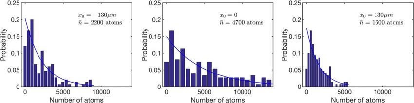
New J. Phys. 20 (2018) 095003 A Vinit and C Raman
averaging over spatial pixels we necessarily included data with different values of n̄ , by ±50% for x0=±130 μm
and ±10% for x0=0. In spite of this, the local exponential character of the distribution clearly persists, and
reveals the thermal statistics of the spin states produced by the quench.
4. Theory
Having directly generated the modes experimentally, we turn now to their theoretical description. We focus our
theory on both q < 0 and q>0 with zero magnetization. Our effort closely parallels that of other experimental
observations of spinor instabilities, with important differences. For example, Bogoliubov theory was applied to a
finite q>0 instability of ferromagnetic F=1, 87Rb spinor BEC [9], as well as to the q=0 instability [20] and
other instabilities [13] of antiferromagnetic F=2 spinor BEC. Broadly speaking, these works have identified
instabilities arising either through bulk modes with a finite wavevector, as in [9, 13], or a specific mode or set of
modes that are resonantly excited at certain values of the quadratic Zeeman tuning parameter [20]. Our studies,
by contrast, explore an intermediate regime. A bulk analysis assuming spatial homogeneity fails to capture
essential features of our observations, particularly the localized instability near the trap center. However, neither
is our experiment dominated by the discrete mode structure of the trap, as the relevant modes along the long axis
of the cigar are too closely spaced for us to resolve. Instead, in our specific experimental geometry, the
inhomogeneous density profile plays an important role in shaping the unstable modes. We uncover these modes
by solving the Bogoliubov equations directly in coordinate space.
Bogoliubov theory was first applied to multi-component (spinor) BEC separately by Ho [36] and Ohmi and
Machida [37]. Following their approach and others [18], one linearizes the spinor Gross–Pitaevskii (GP)
equations (or the corresponding Heisenberg equations of motion for the field operators) about an initial state
that is classical. In our case and several of the examples above, this is a state ψ0 consisting of all atoms in the
m=0 sublevel, with only small corrections δψ±1 describing the populations in m=+1 and −1. Due to the
small ratio c2/c0, we assume that the spin instabilities do not couple strongly to density fluctuations, and thus we
can neglect fluctuations in the m=0 state. The resulting spinor wavefunction may be written as
⎛ 0 ⎞ ⎛dy+1⎞
Y = Y0 + d Y = ⎜⎜ y0 ⎟⎟ + ⎜ 0 ⎟
⎜ ⎟
⎝ 0 ⎠ ⎝dy-1⎠
and the resulting linearized spinor GP equation for m=±1 is [38]:
¶ym ⎛ 2 2 ⎞
i = ⎜- - p (x ) m + qm 2⎟ ym
¶t ⎝ 2M ⎠
+ U (x )(ym + y*-m). (4)
In the above we have simplified the notation to ψm ≡ δ ψm, and assumed a one-dimensional description with
axial coordinate x, so that U (x ) = c2 n0 (x ) = c2∣y0 (x )∣2. To model the data presented in this paper we set the
linear Zeeman term p (x ) = 0 and allow the quadratic Zeeman shift q to vary as a free parameter. We exclusively
study the regime very close to the phase transition, i.e., -U0 q < 0, where U0=c2n0(x=0) and n0(x=0)
is the peak m=0 atom number density at the trap center.
We expand the wavefunctions in a basis of spin excitations, with spatial mode index k and frequency wk :
ym (x , t ) = å uk,m (x ) e-iw t + vk*,m(x ) e+iw t .
k k (5)
k
Note that since the above is actually two equations, one each for m=±1, there will be two spin modes associated
with each spatial mode k. Putting equation (5) into equation (4) and equating terms with equal time-dependence,
we get the Bogoliubov–de Gennes equations:
⎛ 2 2 ⎞
Eu = ⎜ - + q - p (x ) + U ⎟ u + Uv ,
⎝ 2M ⎠
⎛ 2 2 ⎞
- Ev = ⎜ - + q + p (x ) + U ⎟ v + Uu , (6)
⎝ 2M ⎠
where
⎛ uk,1 = u ⎞ ⎛ u k , -1 = v ⎞
⎜ v k, -1 = v ⎟ and ⎜ v k,1 = u ⎟
⎜ ⎟ ⎜ ⎟
⎝ E ⎠ ⎝ -E ⎠
with U≡U(x). The energy eigenvalues of the spin wave modes are E≡Ek. They are collective excitations of the
spin degrees of freedom about the m=0 condensate. Due to the conservation of spin, each of these
8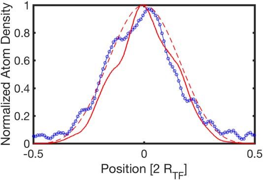
New J. Phys. 20 (2018) 095003 A Vinit and C Raman
Figure 5. Excitation energies of spin modes. Shown is the square of the numerically obtained eigenvalues En; n=1, 2, 3, K for
inhomogeneous density profile (left panel) and homogeneous density (right panel). Eigenvalues are plotted for q=+5 Hz (red, filled
circles), q=0 (blue, open circles) and q=−5 Hz (green, filled circles). E20, the m=±1 components experience a repulsive interaction with
the m=0 condensate. These excitations are very similar to the density modulations of a single component BEC,
where excitations are comprised of atom pairs with equal and opposite momenta ± k, and which are repelled
from the k=0 condensate [39]. For the spin wave case, however, the dynamics are much slower than for sound
waves by the factor c2 c 0 (≈8 for sodium atoms), as first elucidated by Ho [36] and Ohmi and Machida [37].
Thus the lowest excitation frequencies are typically in the range of a few Hz to 10s of Hz.
We find the eigenvalues and eigenvectors of equations (6) using a straightforward matrix diagonalization in
MATLAB [40]. Figure 5 shows the numerical solutions for the energy eigenvalues for some representative
parameters. For q>0 the eigenvalues are real. If q is chosen to be negative, one or more collective modes in
equation (5) has an energy eigenvalue Ek which crosses into the complex plane. This triggers an exponential
growth in the population of those modes, which are linear combinations of the spin states ±1. Thus the
populations y†m ym , for m=±1, also grow exponentially with time, similar to a parametric amplifier [41].
Although we have not written down the Bogoliubov expansion in terms of the field operators ψm, it is
straightforward to do so, and all quantum effects and correlations can be calculated in a straightforward
manner [18].
Before turning to solutions to the equations, we point out some differences between the coordinate and
momentum representations. For uniform systems, Bogoliubov theory is best described in momentum space,
using plane wave modes. One can then write the annihilation operator for a boson with momentum k in terms
of corresponding operators for quasiparticles with momenta k and −k. The Bogoliubov transformation
contains within it, therefore, a direct correlation between quasiparticles of opposite momenta. This correlation
is similar to that obtained in the Bogoliubov diagonalization of the Hamiltonian of a single component weakly
interacting Bose gas [42]. In addition, in the multi-component Hamiltonian, equation (1), the correlation is
between quasiparticles of opposite spin.
In our experiment, where the m=0 condensate has a Thomas–Fermi spatial density profile, an expansion
in momentum eigenstates is not useful. Instead, we have followed the approach of Ruprecht et al in the analysis
of collective excitations of a scalar BEC in a trap [43]. In that case, the Thomas–Fermi density profile led to
collective mode functions that were spatially varying, and which represented modes located inside of or near the
Thomas–Fermi surface.
We will find the same to be true of the collective spin modes for a spinor BEC under harmonic confinement.
An alternate way to view these modes is in terms of standing wave solutions uk,m(x), vk,m(x) for the small
excitations ±1 that are created within the Thomas–Fermi boundaries of the m=0 cloud (see figure 6(A) for an
example). Thus, rather than momentum correlations, as expected for a uniform system, the Bogoliubov analysis
reveals the spatial correlations for particles of opposite spin m=±1, as noted in figure 2 and our earlier work
[4]. The correlations only exist, however, within the domains defined by those modes.
9New J. Phys. 20 (2018) 095003 A Vinit and C Raman
Figure 6. Unstable modes and their spatial profiles. (A) Bogoliubov solutions for U=96 Hz and q=−4.2 Hz. Shown are the
probability distributions of the maximally unstable mode (n=1, no nodes), a less unstable mode (n=6, 5 nodes), and the n=1
mode for the homogeneous density case. (B)–(F) Representative experimental observations of domains nucleated by the instability at
t=20 ms after the quench. Solid lines are the threshold used to determine rms domain sizes. (G) (Right) Calculated rms width of the
maximally unstable eigenvector versus distance to the phase transition point −q. The horizontal line is the value that corresponds to
the experiment. (Left) Histogram of the observed domains for 30 runs of the experiment at q=−4.2 Hz shows an average domain
size that is smaller than that of the lowest mode, suggesting the involvement of higher lying modes n>1.
4.1. Uniform density profile
The case of a uniform m=0 density, U = constant, is a useful point of reference since the solution can be
analytically obtained. The energy spectrum in this case is
Ek = ( k + q)( k + q + 2U ) , (7)
where k = 2k 2 (2M ), k=π/L×n, n=1, 2, 3, K, for excitations in a box of length L=2RTF, where RTF is
the axial Thomas–Fermi radius. The Bogoliubov eigenfunctions are box modes
2 ⎡ np ⎤
fn (x ) = sin ⎢ (x + L 2) ⎥ (8)
L ⎣ L ⎦
10New J. Phys. 20 (2018) 095003 A Vinit and C Raman for ∣x∣ < L 2. For our parameters the ground state energy of the box 1 h ´ 0.05 Hz is smaller than our experimental resolution, so we can assume a quasi-continuous spectrum. Thus for q>0 all eigenvalues are real, while for q
New J. Phys. 20 (2018) 095003 A Vinit and C Raman slightly higher in energy than the even parity ones, but the difference is very small for n
New J. Phys. 20 (2018) 095003 A Vinit and C Raman
develop into something that is spatially localized. For longer times where the m=0 component becomes
depleted, this spatially localized state is no longer stable, but expands into a multi-domain structure.
Indeed, we can see from our experimental data in figure 2 that the instability creates spin structures that are
spatially localized near the center of the Thomas–Fermi region. Through the second order correlation function
we determined the average mode size to be 33 μm, which is in good agreement with the rms width of 35 μm
predicted for the maximally unstable mode uMAX(x). The latter is shown as a horizontal line in figure 6(G), right
panel.
From Bogoliubov theory at q=−4.2 Hz, we estimate that 30 modes have an imaginary component.
Therefore, the maximally unstable mode is not the only active mode in the problem. While the average domain
size, as measured by the normalized second-order correlation function g2(x), is well captured by theory, we still
must understand the varying number and size of the domains measured in the experiment. To uncover these
multi-mode effects, we look at the spread in experimentally observed domain sizes using an rms domain width
analysis. Figure 6, panels (B)–(G), show mode profiles measured at the onset of the instability, t=20 ms, when
the mean population in the ±1 states was 15%. We show 5 separate instances of the experimental quench
sequence that are representative of the variations observed. Shot to shot fluctuations reflected the stochastic
dynamics discussed earlier. By observing peaks in the data, we could determine the rms size of domains
associated with those peaks. We determined these sizes using a simple criterion–the size was the minimum
distance from the peak where the data crossed a threshold value of=e−1/2 of its peak value, as would be
expected for the rms width of a Gaussian function. The threshold is shown as a solid line in the plots. The
preponderance of multi-domain structures makes it clear that multiple modes are present.
Figure 6(G) explores this multi-mode character of the instability by comparing the domain widths
quantitatively. On the right panel we have computed the rms width of the maximally unstable mode obtained
from the Bogoliubov calculation, uMAX(x), versus the final quadratic Zeeman shift ∣q∣ = -q . On the left panel
we show a histogram of the observed rms sizes of the domains for 30 runs of the experiment at q=−4.2 Hz. On
the higher end, the distribution cuts off at a domain size that corresponds well with xrms=35 μm for the lowest
mode, u=uMAX. Nonetheless, domains as small as 15 μm were observed, not much larger than our spatial
resolution of 10 μm, indicating that the quench excited many higher order modes. The tail in the distribution
above 35 μm is most likely caused by mistaken identification of multiple overlapping domains as a single, larger
domain, an example of which is shown in panel (C).
5.2. Dynamical phase
In this later phase, we observe a coarsening of the domains generated in the growth phase. The upper panel of
figure 7 shows the crossover from growth to dynamical phases in the one-dimensional m=−1 density profiles,
which have been plotted against their axial position normalized to the axial Thomas–Fermi radius, RTF. Similar
data were obtained for the m=+1 profile. Each curve is an average of 3 experimental runs normalized to the
peak value at each time step, with each curve displaced by 1 for clarity. The average reduces the effect of
stochastic fluctuations associated with spontaneous domain formation, allowing us to focus on the coarsening
trend—there is a growth in the overall size of the m=±1 clouds with time. As seen in the figure, for short times,
when Bogoliubov theory is still applicable, the density profile grows from the center of the cloud, forming a
localized hump at a time when fpm≈0.05. As time increases, this hump grows in size to envelop the cloud.
Although we can no longer use the unstable Bogoliubov eigenmodes to analyze the dynamical phase, we can
compare our data with numerical simulations. To this end we compute a different rms width, this one pertaining
to the entire m=−1 cloud
ò ∣ u (x )∣2 x 2dx
x rms = (11)
ò ∣ u n (x )∣2 dx
which is shown in the lower panel of figure 7. Here ∣ u (x )∣2 is equal to the measured density profiles shown in the
upper panel of the figure. The width of the density hump is seen to increase with time as the system evolves into
the dynamical phase, exhibiting an overdamped oscillation before reaching a steady-state value of about 0.4RTF.
At t=16 ms the super-Poissonian noise was larger than at later times, and imperfect averaging led to a larger
error bar. Although the coarse cloud size in each of the three interpenetrating quantum fluids, m=0 and
m=±1, has reached a steady-state, the dynamics have not yet halted, as the fraction f± continues to steadily
increase, as seen earlier in figure 1(C). In this later phase of the non-equilibrium behavior micro-domains still
exist and move throughout the cloud. As noted in our earlier work, one can observe a small, local magnetization
density M(x)=n+1(x) − n−1(x). Thus the m=±1 clouds eventually separate from one another [4].
13New J. Phys. 20 (2018) 095003 A Vinit and C Raman
Figure 7. Evolving from growth to dynamical phases. (Above) From bottom to top, experimental traces for the m=−1 state averaged
over 3 shots to coarse grain over domain stochasticity, for times t=16 to 44 ms after the quench in 4 ms intervals. Corresponding
fraction of atoms in the ±1 is written next to each curve. Each curve has been normalized to its peak value and displaced for clarity of
presentation. (Below) Rms width of the density profile versus hold time. Error bars are the standard deviation of the 3 separate
measurements.
14New J. Phys. 20 (2018) 095003 A Vinit and C Raman
5.3. Numerical results
Numerical simulations allowed us to bridge the growth and the dynamical phases of evolution, and to probe the
early part of the growth phase where little experimental data could be obtained. We performed one-dimensional
simulations of the 3 coupled spinor GP equations seeded with noise according to the truncated Wigner
approximation, or TWA. The population dynamics derived from the simulations were reported in our earlier
work [4]. Here we provide more details including the numerically obtained wavefunctions and their temporal
evolution. Our numerical procedure is a straightforward forward time propagation of the equations of motion
using a time-splitting spectral method (see, for example, [44] and references therein). The TWA approximation
is expected to be valid for both short and long times, as long as the initial condition is a classical state [45–48]. To
implement these simulations, as discussed in [4], we assumed a BEC initially at zero temperature and obtained
the initial wavefunction for the m=0 component numerically. Vacuum noise in the m=±1 states was
simulated as classical noise, and we computed the average density, áy†m ymñ, as an ensemble average over 30
separate simulations using different random initial conditions. Vacuum modes with wavelength less than ξspin
are not expected to contribute to the spin instability. Therefore, we imposed a cutoff energy of c2n0, which
resulted in Nv ; 700 virtual particles, while the condensate contained 5×10⁶ particles, similar to the
experimental conditions. To study the early time behavior in the simulations it was also essential to subtract a
constant from the average density = Nv/(2RTF) equivalent to the sum of all virtual particles added, which was
done according to the Weyl representations of the field operators [46].
As mentioned earlier, the experimental data measure the integrated column density n˜(x ) = ò n (x , y , z ) dy dz .
To compare this with a one-dimensional simulated density profile n (x ), we first posit a solution that is separable in
space between axial (x) and transverse (y, z) coordinates:
Ym(x , y , z , t ) = ym (x , t ) x ( y , z ) , (12)
where ψm(x, t) is the simulated wavefunction for spin state m. Since the quench is one-dimensional, we may
assume that the transverse mode function ξ, normalized as ò ∣x∣2 dy dz = 1, is time-independent as the dynamics
are frozen. With the approximation equation (12) and the three-dimensional density distribution
nm (x , y , z ) = ∣Ym∣2 , the measured column density becomes
n˜ m (x ) = ò nm (x, y, z ) dy dz = ∣ym (x, t )∣2
and is identical to the one-dimensional density profile obtained from the simulation. However, for a Thomas–
Fermi BEC, the solution is not strictly separable, as the transverse Thomas–Fermi radius depends on axial
position x. In effect, equation (12) assumes a Thomas–Fermi cylinder rather than a cigar. If the cigar aspect ratio
is very large (70 in our case), the difference between cylinder and cigar is insignificant, particularly since most of
the important quench dynamics occur near the cloud center. However, care must be paid when one approaches
the axial Thomas–Fermi radius, x=±RTF, as there are likely to be quantitative differences.
On the left panel of figure 8, we show the result of the numerical simulations, and on the right pane is shown
the prediction for the ensemble averaged density profile from Bogoliubov theory. Here we have computed
å∣uk∣2 e Gk t where the sum runs over all unstable modes. The growth factor Γk=Im [Ek/h]. The curves have been
normalized in the same manner as for the experiment. At t=0 the exponential factor is 1 for all modes,
resulting in a nearly uniform initial density profile.
Both Bogoliubov and full numerical theories agree with one another during the growth phase of the
dynamics. Moreover, the theory confirms the local density picture discussed earlier, where a uniform
distribution comprised of vacuum fluctuations in all modes becomes narrower with time, eventually becoming
localized near the cloud center. For the Bogoliubov results, at later times the maximally unstable mode, ΓMAX,
begins to dominate, and the curves begin to peak around this mode function, uMAX, which is shown as the
narrow distribution in the uppermost plot of the right pane. Even at a time t=10/ΓMAX, however, the
Bogoliubov density distribution has not fully converged to uMAX, but remains broader. Our experimental data
shows the formation of the localized structure, but not its precursor, the uniform phase, which is hidden in
experimental noise. The uniform phase is, however, captured by the TWA simulations (see the lowest traces of
the left panel).
An interesting artifact in the simulations can also be observed in figure 8, one which illustrates some of the
limitations of the Bogoliubov analysis. The TWA initial condition was taken to be a sum of Bogoliubov
eigenmodes prior to the quench (see the next section for details of these stable modes), with random coefficients.
Since these modes are defined on x Î [−RTF,+RTF], their amplitude goes exactly to zero at the Thomas–Fermi
radius. However, the numerical simulations are not restricted to the Thomas–Fermi volume, but capture the full
details of the cloud’s surface structure, even for ∣x∣ > RTF . Thus at short times in the simulation, the repulsive
interaction between atoms redistributed the m=±1 density from inside to outside of RTF such that as x
approached ± RTF from within the cloud, the Weyl correction was no longer accurate and yielded a negative
density, seen in the lowest traces. Therefore, at short times the m=±1 density should be even more uniform
15New J. Phys. 20 (2018) 095003 A Vinit and C Raman
Figure 8. Average density profiles predicted by theory. Numerical simulations are shown on the left. Bogoliubov theory, equation (5)
is shown on the right, for times t/τMAX=1, 2, K 10, with the maximally unstable eigenvector, ∣uMAX∣2 , shown in the uppermost
graph for comparison. Here τMAX=1/Im(EMAX) is the timescale associated with uMAX. In both panes, each curve has been
normalized to its peak value and displaced for clarity of presentation.
than the simulation suggests. This artifact had no bearing on the simulation at longer times, since the Weyl
correction, which counts only the vacuum fluctuations, was insignificant in comparison with the number of real
particles. Nonetheless, it illustrates the difficulty in describing the details of the dynamics near the Thomas–
Fermi surface.
Finally, an agreement between all 3 density profiles—the experimental data, TWA simulations, and
Bogoliubov theory—was found at a time approaching the crossover from growth phase to dynamical phase. This
data is shown in figure 9. The experiment and TWA curves were taken at a time when the ±1 fractions were
similar, having reached f±1=0.15 and 0.17, respectively. This allowed us to circumvent a factor of 4 difference
observed in the absolute timescale for the quench dynamics between the two, as noted in [4]. These data contain
residual oscillations due to imperfect averaging. The Bogoliubov theory was taken at a time t=10τMAX. All 3
curves are broader than the maximally unstable eigenmode uMAX. Bogoliubov theory should converge to the
maximally unstable eigenmode; however, this only occurs after a sufficiently long time. We observed
convergence at a time t » 100GMAX , by which time in the experiment the m=0 cloud would have been
significantly depleted, violating the Bogoliubov approximation. This provides further confirmation that our
experiment is in a multi-mode regime even during its growth phase, when Bogoliubov theory is valid.
5.3.1. Stable modes
For completeness, we include a discussion of the collective excitation spectrum for q > 0 , although no
experimental data was taken in this regime. Nonetheless, it provides additional insights into the difference
between homogeneous and inhomogeneous cases, particularly as q 0 , the phase transition point. Here the
eigenvalues are all real and positive, and n is a mode index by which they are sorted in increasing order. Similar to
16New J. Phys. 20 (2018) 095003 A Vinit and C Raman
Figure 9. Average density profiles for experiment (open circles), simulation (thick red line), and Bogoliubov theory (dashed line).
Figure 10. Stable spin modes. Shown are Bogoliubov functions u(x) (red) and v(x) (blue) for q=+5 Hz, U=96 Hz, for the
inhomogeneous Thomas–Fermi density profile, whose repulsive potential is shown as a black dashed line. (Below, solid lines) Mode
with the lowest energy n=1. (Above, dotted lines) A higher excitation mode n=9, offset vertically for clarity.
the unstable modes discussed in the previous section these modes also depart from the homogeneous
Bogoliubov solutions, equation (8). Their spatial profile also depends upon q in a manner that was determined
numerically.
The lower graph of figure 10 shows the numerically obtained mode functions, u1(x) and v1(x), for the lowest
energy eigenvalue E1, at a quadratic Zeeman shift of q=+5 Hz. These functions are sharply localized near the
Thomas–Fermi boundary at x/LTF=±1/2, in stark contrast with the homogeneous modes that are delocalized
throughout the Thomas–Fermi region. For increasing n the modes penetrate further into the cloud—for
comparison, the n=9 mode, with even parity, is shown in the upper graph.
We can understand the mode structure for q>0 in terms of the total potential appearing in the Bogoliubov
equations:
⎛ x2 ⎞
U (x ) = c2 n 0 (x ) = c2 n 0 ⎜1 - 2 ⎟ ,
⎝ R ⎠
where n0 is the density averaged over the 2 radial directions of the optical trap. Beyond the Thomas–Fermi radius
we can set U (x ) = ¥, since the harmonic potential increases very rapidly in comparison with the energy scale
c2n0. Figure 10 shows U(x) as a dashed line. It resembles the box potential obtained in the homogeneous case, but
with an additional bump at x=0 that shifts the excitations away from the cloud center and toward the Thomas–
Fermi boundary. This repulsion was discussed earlier as being due to antiferromagnetism—for c2>0 the spin
m=0 and spin ∣m∣ = 1 quantum fluids repel one another. Since the excitations are ±1 atom pairs, their
minimum energy configuration is a localized state at the edge of the cloud.
Crossing the phase transition results in a transformation from stable to unstable behavior of the eigenmode.
This effect is explored in figure 11 for the lowest energy state. Only within a tiny region near the critical point
having a width of 0.1 Hz, does the mode function become delocalized. By contrast, in the homogeneous case the
mode sin π (x+L/2)/L remains the same on both sides of the phase transition, and is always maximum
at x=0.
17New J. Phys. 20 (2018) 095003 A Vinit and C Raman
Figure 11. Transformation of the wavefunction caused by the instability. Shown is the numerically obtained function ∣ u (x )∣2 for the
lowest energy eigenvalue for 100 values of q near the phase transition point, qcrit=−0.005 Hz. The deviation of qcrit from 0 occurs
due to the discreteness of the eigenvalues. The data are scaled to the peak value of ∣ u (x )∣2 at each q for clarity of presentation. For
positive q the excitation is localized at the Thomas–Fermi boundary of the m=0 cloud, while for negative q it is localized in the cloud
center. The transition from the boundary to the center of the cloud occurs very suddenly as q is changed—note that the entire span of q
is only 0.4 Hz in the figure.
6. Conclusion
For spatially extended quantum systems, the study of relaxation toward equilibrium naturally involves the
dynamics of many modes and the flow of energy between them. We have used the second-order correlation
function, g2(x), and statistical analysis of domain widths to reveal the richness of this multi-mode behavior in
quenched antiferromagnetic spinor Bose–Einstein condensates. These approaches, combined with a portfolio of
theoretical tools, have allowed us to span the data from the early, growth phase, to the later, dynamical phase. For
the former case, Bogoliubov theory is a semi-analytical approach which provides much physical intuition.
However, for the latter case we have relied on numerical simulations in order to explain the data. Future work
will explore possible dynamical universality in the long time dynamics, which could provide new analytical
insights beyond the numerical work that has been done here [49].
Acknowledgments
This work was supported by NSF grant No. 1707654.
ORCID iDs
C Raman https://orcid.org/0000-0002-9330-7591
References
[1] Sachdev S 1999 Quantum Phase Transitions (Cambridge: Cambridge University Press)
[2] Langen T, Geiger R and Schmiedmayer J 2015 Ultracold atoms out of equilibrium Annu. Rev. Condens. Matter Phys. 6 201–17
[3] Vinit A and Raman C 2017 Precise measurements on a quantum phase transition in antiferromagnetic spinor Bose–Einstein
condensates Phys. Rev. A 95 011603
[4] Vinit A, Bookjans E M, de Melo C A R and Raman C 2013 Antiferromagnetic spatial ordering in a quenched one-dimensional spinor
gas Phys. Rev. Lett. 110 165301
[5] Bookjans E M, Vinit A and Raman C 2011 Quantum phase transition in an antiferromagnetic spinor Bose–Einstein condensate Phys.
Rev. Lett. 107 195306
[6] Kang S, Seo S W, Kim J H and Shin Y 2017 Emergence and scaling of spin turbulence in quenched antiferromagnetic spinor Bose–
Einstein condensates Phys. Rev. A 95 053638
[7] Stenger J, Inouye S, Stamper-Kurn D M, Miesner H J, Chikkatur A P and Ketterle W 1998 Spin domains in ground-state Bose–Einstein
condensates Nature 396 345–8
[8] Chang M S, Hamley C D, Barrett M D, Sauer J A, Fortier K M, Zhang W, You L and Chapman M S 2004 Observation of spinor dynamics
in optically trapped Rb Bose–Einstein condensates Phys. Rev. Lett. 92 140403
[9] Sadler L E, Higbie J M, Leslie S R, Vengalattore M and Stamper-Kurn D M 2006 Spontaneous symmetry breaking in a quenched
ferromagnetic spinor Bose–Einstein condensate Nature 443 312–5
[10] Black A T, Gomez E, Turner L D, Jung S and Lett P D 2007 Spinor dynamics in an antiferromagnetic spin-1 condensate Phys. Rev. Lett.
99 70403
18New J. Phys. 20 (2018) 095003 A Vinit and C Raman
[11] Liu Y, Jung S, Maxwell S E, Turner L D, Tiesinga E and Lett P D 2009 Quantum phase transitions and continuous observation of spinor
dynamics in an antiferromagnetic condensate Phys. Rev. Lett. 102 125301
[12] Klempt C, Topic O, Gebreyesus G, Scherer M, Henninger T, Hyllus P, Ertmer W, Santos L and Arlt J J 2009 Multiresonant spinor
dynamics in a Bose–Einstein condensate Phys. Rev. Lett. 103 195302
[13] Kronjager J, Becker C, Soltan-Panahi P, Bongs K and Sengstock K 2010 Spontaneous pattern formation in an antiferromagnetic
quantum gas Phys. Rev. Lett. 105 90402
[14] Zhao L, Jiang J, Tang T, Webb M and Liu Y 2015 Antiferromagnetic spinor condensates in a two-dimensional optical lattice Phys. Rev.
Lett. 114 225302
[15] Seo S W, Kang S, Kwon W J and Shin Y I 2015 Half-quantum vortices in an antiferromagnetic spinor Bose–Einstein condensate Phys.
Rev. Lett. 115 015301
[16] Stamper-Kurn D M and Ueda M 2013 Spinor Bose gases: symmetries, magnetism, and quantum dynamics Rev. Mod. Phys. 85
1191–244
[17] Ueda M 2012 Bose gases with nonzero spin Annu. Rev. Condens. Matter Phys. 3 263–83
[18] Kawaguchi Y and Ueda M 2012 Spinor Bose–Einstein condensates Phys. Rep. 520 253–381
[19] Kasevich M A, Riis E, Chu S and DeVoe R G 1989 rf spectroscopy in an atomic fountain Phys. Rev. Lett. 63 612
[20] Scherer M, Lucke B, Gebreyesus G, Topic O, Deuretzbacher F, Ertmer W, Santos L, Arlt J J and Klempt C 2010 Spontaneous breaking of
spatial and spin symmetry in spinor condensates Phys. Rev. Lett. 105 135302
[21] Ockeloen C F, Tauschinsky A F, Spreeuw R J C and Whitlock S 2010 Detection of small atom numbers through image processing Phys.
Rev. A 82 61606
[22] Ketterle W, Durfee D S and Stamper-Kurn D M 1999 Making, probing and understanding Bose–Einstein condensates Bose-Einstein
Condensation in Atomic Gases Proceedings of the International School of Physics ‘Enrico Fermi’ ed M Inguscio et al (Amsterdam:
IOS Press) pp 67–176
[23] Metcalf H J and van der Straten P 1999 Laser Cooling and Trapping (New York: Springer)
[24] Lücke B et al 2011 Twin matter waves for interferometry beyond the classical limit Science 34 773—6
[25] Gross C, Strobel H, Nicklas E, Zibold T, Bar-Gill N, Kurizki G and Oberthaler M K 2011 Atomic homodyne detection of continuous-
variable entangled twin-atom states Nature 480 219–23
[26] Schmaljohann H, Erhard M, Kronjäger J, Kottke M, van Staa S, Cacciapuoti L, Arlt J J, Bongs K and Sengstock K 2004 Dynamics of
F = 2 spinor Bose–Einstein condensates Phys. Rev. Lett. 92 40402
[27] Hanbury Brown R and Twiss R Q 1956 A test of a new type of stellar interferometer on sirius Nature 178 1046–8
[28] Loudon R 1983 The Quantum Theory of Light (Oxford: Oxford University Press)
[29] Esteve J, Trebbia J-B, Schumm T, Aspect A, Westbrook C I and Bouchoule I 2006 Observations of density fluctuations in an elongated
Bose gas: ideal gas and quasicondensate regimes Phys. Rev. Lett. 96 130403
[30] Jeltes T et al 2007 Comparison of the Hanbury Brown–Twiss effect for bosons and fermions Nature 445 402–5
[31] Perrin A, Bücker R, Manz S, Betz T, Koller C, Plisson T, Schumm T and J Schmiedmayer 2012 Hanbury Brown and Twiss correlations
across the Bose–Einstein condensation threshold Nat. Phys. 8 195–8
[32] Weiner R M 2000 Introduction to Bose–Einstein Correlations and Subatomic Interferometry (Chichester: Wiley)
[33] Kaufman A M, Tai M E, Lukin A, Rispoli M, Schittko R, Preiss P M and Greiner M 2016 Quantum thermalization through
entanglement in an isolated many-body system Science 353 794–800
[34] Bookjans E M, Hamley C D and Chman M S 2011 Strong quantum spin correlations observed in atomic spin mixing Phys. Rev. Lett. 107
210406
[35] Mias G I, Cooper N R and Girvin S M 2008 Quantum noise, scaling, and domain formation in a spinor Bose–Einstein condensate Phys.
Rev. A 77 023616
[36] Ho T-L 1998 Spinor Bose condensates in optical traps Phys. Rev. Lett. 81 742
[37] Ohmi T and Machida K 1998 Bose–Einstein condensation with internal degrees of freedom in alkali atom gases J. Phys. Soc. Jpn.
67 1822
[38] Saito H and Ueda M 2005 Spontaneous magnetization and structure formation in a spin-1 ferromagnetic Bose–Einstein condensate
Phys. Rev. A 72 23610
[39] Pitaevskii L and Stringari S 2003 Bose–Einstein Condensation (International Series of Monographs on Physics) (Oxford: Clarendon)
[40] Matlab The MathWorks, Inc., Natick, Massachusetts, United States
[41] Walls D F and Milburn G J 2008 Quantum Optics 2nd edn (Berlin: Springer)
[42] Pethick C J and Smith H 2002 Bose–Einstein Condensation in Dilute Gases (Cambridge: Cambridge University Press)
[43] Ruprecht P A, Edwards M, Burnett K and Clark C W 1996 Probing the linear and nonlinear excitations of Bose-condensed neutral
atoms in a trap Phys. Rev. A 54 4178–87
[44] Bao W, Jaksch D and Markowich P A 2003 Numerical solution of the Gross–Pitaevskii equation for Bose–Einstein condensation
J. Comput. Phys. 187 318–42
[45] Blakie P B, Bradley A S, Davis M J, Ballagh R J and Gardiner C W 2008 Dynamics and statistical mechanics of ultra-cold Bose gases using
c-field techniques Adv. Phys. 57 363–455
[46] Polkovnikov A 2010 Phase space representation of quantum dynamics Ann. Phys., NY 325 1790–852
[47] Sau J D, Leslie S R, Stamper-Kurn D M and Cohen M L 2009 Theory of domain formation in inhomogeneous ferromagnetic dipolar
condensates within the truncated Wigner approximation Phys. Rev. A 80 23622
[48] Barnett R, Polkovnikov A and Vengalattore M 2011 Prethermalization in quenched spinor condensates Phys. Rev. A 84 23606
[49] Karl M, Cakir H, Halimeh J C, Oberthaler M K, Kastner M and Gasenzer T 2017 Universal equilibrium scaling functions at short times
after a quench Phys. Rev. E 96 22110
19You can also read