High-fidelity CFD Workshop 2021 Inviscid Strong Vortex Shock Wave Interation
←
→
Page content transcription
If your browser does not render page correctly, please read the page content below
High-fidelity CFD Workshop 2021
Inviscid Strong Vortex Shock Wave Interation
Chongam Kim: chongam@snu.ac.kr
February 11, 2020
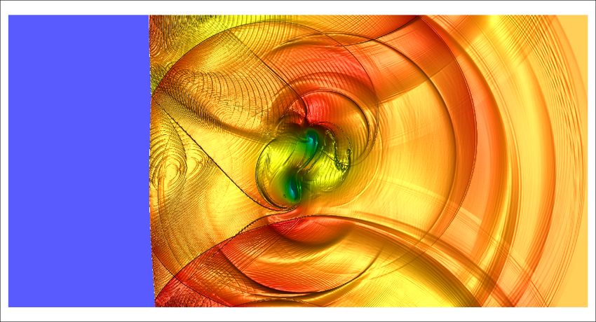
Figure 1: Density contour of the problem
1 Overview
This case is designed to verify that a scheme can capture complex physical phenomena resulting
from the interaction between a strong vortex and a shock wave. This is a two-dimensional unsteady
inviscid flow including multiple shock discontinuities. When the strong vortex and the strong shock
wave encounter, considerable distortion of shock structure occurs, followed by the generation of
linear and non-linear waves propagating onto the downstream flow fields. Two distinctive physical
phenomena can be observed in this problem. First, the strong vortex is split into two separate
vortical structure due to the compression effects of the shock passage. The post-shock vortical
structure depends strongly on the relative strength of the shock and the vortex. Second, cylindrical
acoustic wave structure appears on the downstream side of the stationary shock. The sound waves
centered on the moving vortex core are partly cut off by the shock wave. As a result, alternating
expansion and compression regions are observed. For more details, see ?.
1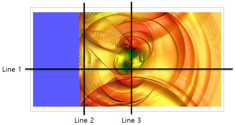
High-fidelity CFD Workshop Scitech 2021                Inviscid Strong Vortex Shock Wave Interaction

                                   Figure 2: Problem description

2    Computational Mesh
Two types of meshes, namely RQ (Regular Quadrilateral) and IM (Irregular Mixed), are provided.
Each mesh is named after its type and the reciprocal of its mesh size. The set of meshes is provided
as follows.

    • RQ (Regular Quadrilateral): RQ100, RQ200, and RQ300

    • IM (Irregular Mixed): IM100, IM200, and IM300

     Simulations with above meshes are mandatory, but results with other types of meshes will be
also welcomed. All types of meshes are provided in GMSH script files (.geo) for unstructured-grid-
based solvers. Participants can generate appropriate GMSH grid files (.msh) by using the script
files and the GMSH program. Read the instructions (Readme.txt) provided in the mesh files. In
addition, RQ type meshes are provided in CGNS grid files (.cgns) for structured-grid-based solvers.
Participants can directly use the CGNS grid files without any pre-processing.
     At the initial state, the stationary shock is exactly aligned with the meshes. No local adaptive
mesh refinement around the shock is applied. Substantial grid perturbation effects may be observed
near the shock wave, particularly when the vortex is passing through the shock wave.

3    Problem Description
To model the flow physics of the strong vortex-shock interaction, the flow is assumed to be governed
by the non-dimensionalized 2-D Euler equations. The system is closed by the equation of state for
air (an ideal gas with the ratio of specific heats, γ = 1.4).
    Initially, the flow fields contains a stationary shock with Ms = 1.5 and a strong vortex with Mv =
0.9. The shock is located at x = 0.5, and the center of the vortex is located at the point (xc , yc ) =
(0.25, 0.5). The upstream flow quantities are specified by (ρu , uu , vu , pu ) = (1.0, 1.775, 0.0, 1.0),
except for the vortex. The vortex rotates counter-clockwise with the angular velocity given below.

                                                   2
High-fidelity CFD Workshop Scitech 2021 Inviscid Strong Vortex Shock Wave Interaction
Figure 3: Selected lines to evaluate computed solutions (t = 0.7)
r
vm a ,
if r ≤ a,
b2
vθ = vm a r− , if a < r ≤ b,
a2 −v2
r
0, if r > b.
Here, r is the distance from the vortex core (xc , yc ), and (a, b) = (0.075, 0.175). vm is the
√
maximum angular velocity, which occurs at r = a. We take Mv = vm / γ as a measure of the
vortex strength. The flow quantities of the downstream (ρd , ud , vd , pd ), i.e. on the right side of the
stationary shock, are determined from the upstream quantities with the stationary shock condition.
The left boundary at x = 0 and the right boundary at x = 2 are considered as a supersonic inlet
and a subsonic outlet, respectively. The upper and lower sides are treated as wall boundary. The
target time for numerical simulation is t = 0.7. See Fig. 2 for the summary of the problem setup.
Detailed procedures to initialize the flow fields are described in Appendix.
4 Data Submission
This flow is highly unsteady and complex with multiple shocks, which poses severe restriction on
conventional order tests. The quality of submitted solutions is thus evaluated by reference solutions
obtained on extremely fine meshes.
For some or all of the given mesh types (RQ and IM), participants should submit their results
as follows. Three specific lines are considered as shown in Fig. 3. Specific description for each line
is given below.
h 2
• Line 1: Pi = (xi , α + ), where xi = 2 + (i − 1) × h, h = N, i = 1, . . . , N
h 1
• Line 2, 3: Pi = (β + , yi ), where yi = 2 + (i − 1) × h, h = N, i = 1, . . . , N
Here, = 0.0001 is added to avoid the overlap with cell interfaces. Each line is defined as follows:
3High-fidelity CFD Workshop Scitech 2021 Inviscid Strong Vortex Shock Wave Interaction
• Line 1: (α, N ) = (0.4, 8000)
• Line 2: (β, N ) = (0.52, 4000)
• Line 3: (β, N ) = (1.05, 4000)
According to the type of solver, participants should submit either cell-averaged solutions or higher-
order solutions at equidistant points Pi along three lines.
• Cell-averaged solutions: Π0 ρk |Pi , where Pi ∈ Tk .
• Higher-order solutions: Πm ρk |Pi , where Pi ∈ Tk for Pm -approximated methods.
Here, ρk is the density distribution on the cell Tk , and Πm indicates a projection onto a polynomial
space of degree m.
Moreover, participants should submit two contour images of the Schlieren variable given as:
ln(1+ k ∇ρ k)
Sch =
ln10
The first image should cover the entire domain [0, 2] × [0, 1], and the second image should
cover the domain of [0.9, 0.12] × [0.330.63] for resolving vortex structures. Both images are 50
equally spaced Schlieren contours in grayscale from 0.05 to 2.4, where the darker colors indicate the
higher values. Participants should provide cell-averaged values and/or sub-cell distributions. When
submitting contour images, specify (cell-averaged and/or sub-cell) contours and describe detailed
plotting procedures.
5 Appendix: Initialization of Flow Fields
Implement S1 to S6 step-by-step in order to initialize the computational flow fields.
S1. Calculate the downstream conditions (ρd , ud , vd , pd ) by using the condition for the stationary
normal shock and the given upstream conditions (ρu , uu , vu , pu ) = (1.0, 1.775, 0.0, 1.0), as follows.
ρu ud 2 + (γ − 1)Ms2 pd 2γ
= = , =1+ (M 2 − 1), vd = 0.0,
ρd uu (γ + 1)Ms2 pu γ+1 s
with Ms = 1.5 and γ = 1.4.
S2. Initialize the computational domain outside the vortex with the given upstream conditions
(ρu , uu , vu , pu ) and the computed downstream conditions (ρd , ud , vd , pd ).
S3. Calculate the velocity field (uvor , vvor ) inside the vortex by superposing the upstream velocity
conditions (uu , vu ) and the tangential velocity field (vθ ) given below. Here, r is the distance from the
vortex core (xc , yc ) = (0.25, 0.5), and (a, b) = (0.075, 0.175) is used. vm is the maximum tangential
√
velocity, which occurs at r = a. We take Mv = vm / γ as a measure of the vortex strength, and
Mv = 0.9 in this computation.
4High-fidelity CFD Workshop Scitech 2021 Inviscid Strong Vortex Shock Wave Interaction
r
vm a ,
if r ≤ a,
a b2
vθ (r) = v r− , if a < r ≤ b,
m a2 −v2
r
0, if r > b.
and therefore
uvor = uu + x − component of vθ ,
vvor = vu + y − component of vθ .
S4. In order to calculate the temperature field (Tvor (r)) inside the vortex, integrate the following
ODE obtained from the normal momentum equation with the centripetal force, as follows.
b b
γ − 1 vθ (r)2 γ − 1 vθ (r)2
Z Z
dTvor (r) dTvor (r)
= → dr = dr
dr Rγ r r dr r Rγ r
Here, R is the gas constant. The above relation is integrated using vθ (r) in S3 with Tvor (b) = Tu
S5. Using the isentropic relation provided below, calculate the density and the pressure field
(ρvor , pvor ) inside the vortex. ρu , pu and Tu are the upstream conditions as references.
1 γ
Tvor (r) γ−1 Tvor (r) γ−1
ρvor (r) = ρu , pvor (r) = pu
Tu Tu
S6. Using the computed density, velocity, and pressure fields, (ρvor (r), uvor (r), vvor (r), pvor (r)),
initialize inside the vortex.
5You can also read