High resolution TCSPC imaging of diffuse light with a one-dimensional SPAD array scanning system

High resolution TCSPC imaging of diffuse light
 with a one-dimensional SPAD array scanning
 system
 E. P. M C S HANE , 1,2,* H. K. C HANDRASEKHARAN , 1 A. K UFCSÁK , 2
 N. F INLAYSON , 2,3 A. T. E RDOGAN , 3 R. K. H ENDERSON , 3
 K. D HALIWAL , 2 R. R. T HOMSON , 1,2 AND M. G. TANNER 1,2
arXiv:2204.07582v1 [physics.ins-det] 15 Apr 2022

 1 Scottish Universities Physics Alliance, Institute of Photonics and Quantum Sciences, Heriot-Watt
 University, Edinburgh, UK
 2 Translational Healthcare Technologies Group, Centre for Inflammation Research, Queen’s Medical
 Research Institute, University of Edinburgh, Edinburgh, UK
 3 Institute for Micro and Nano Systems, University of Edinburgh, Edinburgh, UK
 * epm1@hw.ac.uk

 Abstract: We report a time-resolved single photon counting (TCSPC) imaging system based on
 a line-scanning architecture. The system benefits from the high fill-factor, active area, and large
 dimension of an advanced CMOS single photon avalanche diode (SPAD) array line-sensor. A
 two-dimensional image is constructed using a moving mirror to scan the line-sensor field-of-view
 (FOV) across the target, to enable the efficient acquisition of a two-dimensional 0.26 Mpixel
 TCSPC image. We demonstrate the capabilities of the system for TCSPC imaging and locating
 objects obscured in scattering media - specifically to locate a series of discrete point sources
 of light along an optical fibre submerged in a highly scattering solution. We demonstrate that
 by selectively imaging using early arriving photons which have undergone less scattering than
 later arriving photons, our TCSPC imaging system is able to locate the position of discrete point
 sources of light than a non-time-resolved imaging system.

 © 2022 Optica Publishing Group under the terms of the Optica Publishing Group Publishing Agreement

 1. Introduction
 Two-dimensional single-photon detector arrays have been used to study time-resolved light
 passage through highly scattering media for medical imaging and spectroscopy [1, 2]. In many
 cases, the light capturing ability of the imaging system is limited by detector characteristics
 such as fill-factor and total active area [3]. This is often the case in 2D single-photon avalanche
 diode (SPAD) arrays with integrated timing electronics, routinely deployed for time-resolved
 imaging due to their single-photon detection capability and high temporal resolution. This
 work presents the use of an alternate time-resolved imaging arrangement, applying a SPAD
 line array together with an imaging system which exploits one-dimensional (1D) scanning to
 form a two-dimensional (2D) image. One-dimensional sensors can offer improved light capture
 ability over 2D sensors through higher fill-factor and larger active area designs [4], as discussed
 in section 2.1. We implement a 512 × 1 pixel CMOS-SPAD line array [5], combined with
 a scanning optomechanical element to form a camera-like imaging system. This sensor and
 previous design iterations have been applied elsewhere for time-resolved spectroscopy [6], optical
 coherence tomography [7] and pH sensing [8]. Photon arrival timing electronics are integrated
 within the CMOS sensor architecture for full time-correlated single-photon counting (TCSPC)
 measurements [9]. Unlike many conventional 2D CMOS-SPAD imaging arrays, this line sensor
 boasts a high SPAD fill-factor (active detector area 28.2% of total array area) as the integrated
 control electronics are placed off-pixel. Each pixel comprises 16 grouped SPADs to increase the
 photon capture area. The 512-pixel line-sensor defines the number of pixels in the acquired image

along one axis, with number of pixels in the orthogonal axis dictated by a computer-controlled
scanning element used to sweep the sensor across the FOV in the second axis. The advantage
of this approach over using a 2D imaging detector array is that we effectively create a high
resolution, large format imaging system, a 12 mm line (dimension of the sensor) combined with
the arbitrary scanning positions used. While the need to scan in the second axis adds an overhead
to image formation, this is more than compensated for by the ability to use larger optics for
efficient light collection in a stand-off imaging modality relative to those appropriate when using
typically smaller 2D detector arrays.
We outline the design and imaging ability of this scanning imaging system and demonstrate
application to diffuse photon imaging of light emitted from discrete point sources submerged
within a highly scattering phantom. When imaging with full TCSPC capability, the locations
of a series of sequentially observed light sources are determined. The controlled illumination
required to carry out this experiment is provided by a bespoke optical fibre probe machined using
ultrafast laser ablation techniques, offering multipoint illumination at many discrete locations
along the device length [10]. These two systems operating in tandem recover the location of 18
discrete point sources of light to track the otherwise obscured device length. We suggest the
ability to locate fibre devices deep within scattering media is relevant to medical device location
as previously described [11], we build upon this by offering improved light detection capability
and device path observation rather than a single point. The improved time-resolved imaging of
diffuse photons has application in further environments [12–15].

2. CMOS-SPAD line scanning imaging system
2.1. CMOS-SPAD line sensor
Line sensor architectures generally achieve higher fill-factors than 2D sensors, defined as the
ratio of photo-sensitive area to overall focal plane array area [16]. A higher fill-factor can
vastly improve the overall detection efficiency of a given system, and in this case, the fill factor
improvement from a previously used 2D system (1.5% [17]) to the line scanning imaging system
(28.2% [5]) is significant. Each line-sensor pixel contains 16 individual SPAD detectors orientated
in an 8 × 2 sub-array format with a combined output. Individual detectors within a pixel can be
optionally disabled in accordance with their characteristic background to maximise overall pixel
signal to noise performance, allowing the user to remove the contribution of the highest noise
SPADs in each pixel across the array. The sensor architecture contains two sets of 512-pixel
arrays optimised for blue and red wavelength ranges [5], here we use the longer wavelength
sensitive SPADs most appropriate for the near-infrared "optical window" of biological tissue near
800 nm [18], appropriate for a range of biophotonic applications. Examples of other recently
developed SPAD line sensors can be found elsewhere [19–21].
Single-photon detection timing is recorded with approximately 50 ps time stamping and 150
ps jitter on each pixel. Alternatively, the detector can operate in fast non-time-resolved photon
counting or on-chip histogram creation modes suitable for other applications. Each line-sensor
pixel is 116.365 (height) × 23.78 (width) leading to a total array length of 12.175 mm.
The total size of the die in which the detector is cast is 12.648 mm × 1.990 mm in its long and
short axis respectively. Owing to the larger length of this line sensor relative to the edge length
of many 2D CMOS-SPAD arrays, larger optics can be integrated within the imaging system.
Recent 2D imaging technologies have achieved impressive pixel numbers [22, 23]. Rather than
comparing to all developments, we consider one such sensor ‘QuantiCam’ [24] containing 192
× 128 single SPAD pixels, totalling 24,576 SPADs each with active area 22 2 . The total
active area of the QuantiCam is 557,568 2 . Meanwhile, the sensor used in this work has 512
pixels of 16 SPADs totalling 8,192 SPADs for both the blue and red wavelength range optimised
arrays with total active areas of 571,091 2 and 399,512 2 respectively. In each case we

see that the total active area of the line-sensor is comparable to that offered by an array such as
QuantiCam. An initial assumption is that these sensors would have similar photon counting
capability if used with identical optical systems. However, significant in a widefield imaging
application is the total chip dimension. The 12.175 mm dimension of the line sensor (compared
to 3.2 × 2.4 mm chip dimension for QuantiCam) gives a "large format" sensor, for which larger
optics can be used at a moderate working distance: here we use a 1-inch lens, with a numerical
aperture of 0.5, at approximately 61 cm working distance to achieve a 30 cm FOV. Smaller sensor
formats demand the use of a shorter focal length and thus (assuming similar NA) a smaller
aperture lens at this working distance to achieve this FOV. As such, the light gathering power
or ”etendue” using a large format sensor is much increased, allowing greater practical photon
collection per second from a real scene. This is in addition to the discussed advantages of a large
number of reconstructed image pixels, e.g. 512 × 512 = 262,144, an order of magnitude greater
than QuantiCam. We have compared to QuantiCam as this chip has similar characteristics and
was developed at a similar time to the line sensor used here. In this rapidly advancing field,
higher pixel numbers and active areas are being achieved, although sometimes at the cost of
lacking full TCSPC capability [22]. We suggest that as line format sensors similarly develop, the
potential advantages for imaging we describe should still be considered when comparing the
newest technology.

2.2. Imaging system design
A scanning mirror element sweeps the sensor FOV in the imaging axis orthogonal to the SPAD
line array axis, achieving a 2D image composed of a series of sequentially acquired slices.
To match the sensor pixel number requires 512 image slices in the second axis, resulting in
a 0.26 Megapixel image. For a defined FOV, this offers improved image sampling relative to
most 2D CMOS-SPAD imaging arrays. The scanning element consists of a two-inch reflecting
mirror (Thorlabs, PF20-03-G01) mounted upon a rotation mount (Thorlabs, DDR25/M), offering
high-speed movement (1800◦ /s) and computer control [25]. In principle this rotational element
can scan a typical 30 cm dimension secondary axis (equating to an approximate total scan angle
of 16◦ ) in 9 ms. Data acquisition is synchronised with mirror movement to automatically build
image frames. A one-inch diameter lens (Thorlabs LA1951-B) mounted within an adjustable
mount (Thorlabs SM1Z) achieves a 30 cm field of view along the line sensor axis at a working
distance of 61 cm. The mirror is rotated a total of 16◦ to achieve a secondary axis with FOV equal
to that obtained in the sensor hardware axis. The system also integrates a 2D CMOS imaging
sensor (Thorlabs Kiralux, CS126CU) for conventional imaging of scenes when the mirror is
rotated 90 degrees.

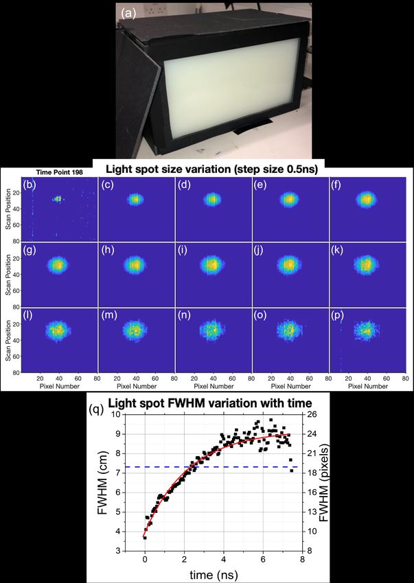
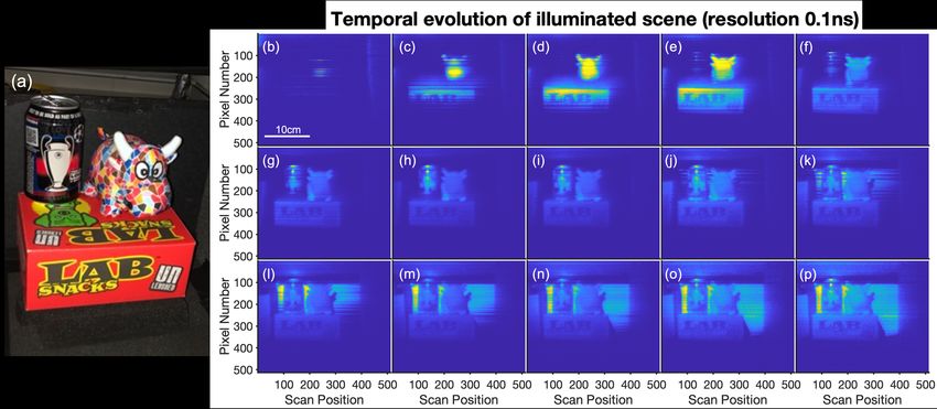
Fig. 1. Optical design and housing of the scanning imaging system. (a) Outline
 of key system optical components. (b) Render of the imaging system housing and
 major internal components using computer aided design software. The housing was
 subsequently realised through 3D-printing, then foil lined, allowing the scanning
 imaging system prototype to be applied within ambient light scenarios.

Figure 1(a) outlines the key optical components of the system. Figure 1(b) displays computer-
aided design renderings (Solidworks) of the imaging system outlining key system components.
System hardware has been placed within a bespoke foil lined housing to mitigate against spurious
light leakage, including an internal baffle with a narrow-band filter centred at 780 nm (Semrock,
780/12 nm BrightLine) directly in front of the sensor to limit incident ambient light being
recorded during imaging. The housing containing these components allows the imaging system
to be portable, rugged, and applied in off-the-bench scenarios. The total size of the system was
minimised whilst also containing all system components, only requiring external connection for
computational control and power, and to provide the TCSPC trigger signal. The system housing
was developed using computer aided design package Solidworks and 3D-printed to specification.

2.3. High-resolution imaging
To demonstrate the TCSPC imaging capabilities of our system, we imaged a scene composed
of several detailed objects which were flood illuminated from a fibre laser source (785 nm,
0.5 mW, 96 ps pulse duration) which was placed adjacent to the imaging system. Photons
reflected/scattered from the scene were collected for a total exposure time of 10.24 seconds,
encapsulating the entire measurement of all image strips. The total exposure time was limited by
requiring sufficient photon counts to achieve satisfactory signal-to-noise, and not by scanning
electronics. Each image strip was produced with a frame exposure time of 20 (in which
a single photon can be counted and time tagged on each pixel), and 1000 frames sequentially
acquired at each mirror position. Time-resolved images separated by a temporal step of 0.1 ns
can be seen within Figure 2(b-p), a subset of the frames acquired at 50 ps separation. Details such
as the well-defined text can be clearly distinguished, and the 3D profile of the target objects is
represented frame to frame. This clarity of imaging is achievable with high image sampling due
to the effective high pixel density created by sweeping the line sensor across the target. Imaging
resolution is 0.59 mm based on pixel density (30 cm / 512 pixels), imaging a test target confirmed
imaging resolution is limited by pixel pitch rather than optical system resolution. Within Figure
2 the presence of some fixed pattern noise is apparent, these effects are due to pixel-to-pixel

variation in DCR and sensitivity. Sensitivity was not calibrated and corrected for within this
imaging, however correction could be applied in future applications.

 Fig. 2. TCSPC imaging of a flood illuminated scene. Objects are disambiguated in
 time, revealed only as the illumination photons encounter them within the measurement
 window. (a) Camera image of the scene. (b-p) Images at increasing times within the
 measurement window (step size between images of 0.1 ns). (See visualisation 1).

In the scene above each tile shows the light detected at a specific time-point within the measurement
window, the series describes the light washing over the scene. Objects placed closer to the light
source are illuminated earlier with details behind becoming visible later. For example, two of the
objects are illuminated at slightly earlier times, e.g. (b)-(d), in contrast to the light pulse reaching
the back of the scene later in the time window, e.g. (k)-(o). Fine temporal resolution can be used
to selectively observe different objects within the field. Well established analysis could be used
to perform depth imaging or light detection and ranging (LIDAR) [26–28], including imaging
partially obscured objects [29].

3. Time-resolved diffuse photon imaging
Time-correlated imaging can be used to observe the progression of light through highly scattering
media for imaging applications [12–15]. For example, time-resolved imaging of light emission
from a point source suspended within scattering media has the potential to infer the location
of that source [11]. As photons pass through a diffusive phantom media, they undergo many
scattering interactions with constituent particles. This acts to spread the pulse of photons in both
space and time. An imaging system focused upon the edge of a phantom, where photons exit to
free-space, will observe a region of scattered light emission. Temporal observation of photons
emerging from the medium will show a significant variation with respect to an unperturbed laser
pulse travelling through a media with minimal scattering. Many scattering events will result in a
time broadened laser pulse, the peak of which will correspond to the modal optical path length of
photon transit through the media, with associated transit time at which the greatest number of
photons will arrive at the sensor. Photons emerging relatively late and early (with respect to the
temporal peak) within the measurement window are considered to have statistically undergone
more and less scattering respectively. More scattering events generally act to increase the optical
path length travelled, and therefore delay photon transmission.

At early times in the measurement window the subset of photons emerge that have undergone
minimal scattering (relative to the later arriving photon cloud) having taken the shortest optical
path from the source through the phantom [30]. However, fast transit along a short optical
path is also possible with many scattering events, provided scattering is in a forward direction,
approximately maintaining the same direct path. This is similar in practice to photons with few
scattering events, also following such a direct path. Many varieties of biological media exhibit
large amounts of anisotropic scattering, such that scattered photons traversing through the media
have a high probability of being forward-scattered [31], consistent with the theory of scattering
from spherical particles. As such, more photons have an approximately direct path than just
those minimally scattered. Photons emerging first from the scattering medium (early arriving
photons at the imaging system detector, “early-photons”) can be temporally separated during
data processing from the later arriving photon cloud. Such early-photons represent the exit point
of photons that have taken the most direct path through the scattering medium. This location can
be used to infer the obscured light source position [11], as studied below.
A scattering phantom composed of homogenised semi-skimmed milk (a colloidal lipid suspension)
provided a scattering coefficient comparable to that of biological tissue. The broadband optical
properties of milk are dominated by scattering, characterisation of the optical properties of milk
along with information on photon interaction with lipid particles can be found elsewhere [32]. A
phantom solution of 1:4 parts semi-skimmed milk to water provided a phantom with a reduced
scattering coefficient of approximately 10 cm−1 , comparable to the 9 cm−1 of muscle tissue
reported within [33]. A bespoke polymer optical fibre was anchored in a fixed location to provide
highly non-directional point source illumination (785 nm) [10]. The phantom tank dimensions
were 40 × 25 × 25 cm (25 L) with illumination suspended approximately 15 cm from the
imaged side of the tank. Laser power launched into the fibre was 4.5 mW, based upon previous
measurements of light emission by Chandrasekaran et al. we estimate emission from a discrete
point on the fibre of 2.5-3.3 mW.

Fig. 3. Temporal evolution of light emitted from a single obscured point source located
within the phantom. (a) Camera image of the scattering phantom described further
within the text. (b-p) Variation of the imaged photon spot size with time. Each tile is
separated in time by 0.5 ns, ten 50 ps time bin steps. (q) Temporal variation in the full
width half maximum of a vertical strip taken through the imaged spot (a subset of which
are shown in Figure 3(b-p). The FWHM of the spot is seen to increase dramatically.
The red trend line is plotted as a guide to the eye, proportional to (1 − − ). The
FWHM of an all-photon image containing all light detected summed together is plotted
as the blue horizontal line.

The exposed side of the tank was imaged with the system described, with a per frame exposure
time of 100 s for 2000 frames in each of the 160 image slices, leading to a total image acquisition
time of 32 seconds. For the purpose of this experiment, recovered images were down sampled
to improve signal to noise, hence the reduction in pixel density observed in Figures 3, 4 and 5
with respect to the pixel density presented in Figure 2. The observed signal evolution from a
point suspended within the scattering phantom is presented within Figure 3(b-p). The light spot
size varies significantly within the measurement window as photon scattering progresses with
the full width at half maximum (FWHM) of the imaged light spot increasing as presented in
Figure 3(q). The FWHM of the non-time-resolved sum of all light within the measurement time
window has been plotted as a horizontal line. The photon emission spot is, as expected, more
tightly located at early time points than both the non-time-resolved “all-photon” sum and the
later arriving photon cloud.
From these simple experiments it is clear that the exit locations of the later arriving photons are
less representative of the position on the tank surface that is closest to the source. Therefore, we
apply an early-photon processing rationale to estimate the light source location with increased
confidence. However, this homogeneous model is a poor mimic of biological tissue, and the later
arriving photon cloud also provides a clear suggestion of the original source location. This would
not be the case with increasing amounts of optical complexity in biological models.

3.1. Device length location in a scattering phantom
The scanning imaging system was applied to observe diffuse light emitted from many discrete
point sources submerged within the scattering phantom. The combined spatial and temporal
resolving capability was utilised to infer the spatial location of a series of light emission points
along a polymer optical fibre device. The bespoke multi-point emission optical fibre provided
known illumination from eighteen discrete selectable points as outlined within [10], placed along
the fibre device length with a pitch of 2 cm. The points were sequentially illuminated and imaged
while submerged in the scattering phantom, with the fibre curving in an arc across the FOV. Early
and late emerging photon images are compared in Figure 4 for nine of the emission points, while
the fibre path is analysed in Figure 5, including the path of the fibre observed without a scattering
medium.
We apply TCSPC imaging to locate each light source submerged within the phantom by analysing
the time-resolved images of each point (comparable to that seen within Figure 3(b-p)), taking
the earliest light as most representative of the location. We track the fibre device path across
the phantom, as the discrete point sources span the device length. Image acquisition, control of
illumination point, and data processing are automated to predict the spatial location of each light
source on a point-to-point basis. Data processing (not in real time) proceeds as follows. Firstly,
the peak of photon counts of the TCSPC histogram (detailing the distribution of photon arrival
times) was found from each illumination point data set. The time-point at which comparatively
earlier photons were detected within the measurement window was then defined as when the
signal reached 10% of the peak photon counts. The image of the photon spot at this early arrival
time was extracted, and the centroid (arithmetic mean position) of the bright region was taken
as an estimate of the light source location. It should be noted, earlier time points given by a
lower photon threshold produce a smaller photon cloud image for determining source location.
However, here a compromise was made to provide sufficient signal to noise to allow reliable
automatic processing of data. In future more advanced processing of earlier photon arrivals, or
indeed analysis including later photon arrivals [15], could be employed.

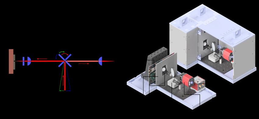
Fig. 4. Early- and all-photon images of light emitted from nine discrete fibre point
 sources submerged within the phantom. The known device path (imaged in the
 absence of scattering particles) has been overlaid on top of each data-set in black. (a-i)
 Early-photon and (j-r) all-photon images

Figure 4 displays the early-photon and non-time correlated all-photon images of light emerging
from the tank emitted by nine discrete point sources along the fibre device length. The early-
photon emission spots are observed to closely track the arc of the optic fibre, with the observed
emission tightly confined to a small area, whereas the all-photon images show larger emission

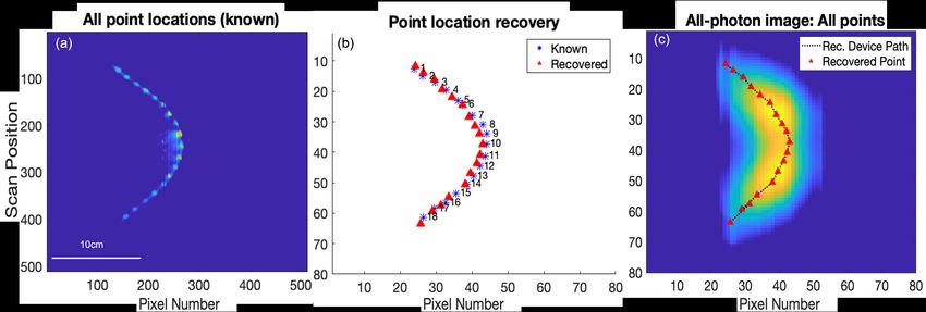
regions. The recovered locations were compared to the known light-source locations, imaged in
the absence of scattering elements within the phantom (Figure 5(a)). The recovered and known
locations are shown within Figure 5(b), where all point locations (blue stars) were recovered in
proximity to the known locations (red triangles). The average deviation between the two locations
across the dataset was small, at approximately 0.51 cm (1.37 image pixels of Figures 5(b,c)).

 Fig. 5. Obscured device tracking using TCSPC imaging. The known emission point
 locations (imaged in the absence of scattering particles) have been recovered using
 the early-photon processing rationale outlined above. (a) Combined visualisation of
 eighteen point sources across the phantom, imaged in the absence of scattering particles.
 (b) The locations recovered using automated processing (red triangles) along with the
 known locations from (a) (blue stars). (c) Combined image of all light emitted from all
 sources on the optical fibre, compared to the recovered locations. (Note: The resolution
 in image (a) is higher than the binned images used for location recovery processing).
 (See visualisation 2).

Figure 5(c) has been created using a summation of the eighteen all-photon images for each point
source (e.g. the images in Figure 4(j-r)). When all images are overlaid in this fashion a poor
correlation to the recovered locations (plotted in red) is observed, representing attempting to
locate the device with neither the bespoke controlled fibre illumination nor time-resolved imaging
capability. The authors note there may be some systematic variation in the recovered and known
locations, which may be a result of boundary effects at the edge of the tank.
The scanning imaging system and multi-point fibre device used in combination demonstrate
device tracking within the highly scattering phantom with sub-centimetre accuracy. The high
spatial resolution of the imaging system is used to provide discrete information of light-source
location over centimetre incremental steps throughout the FOV, and the high temporal sensitivity
of time-stamping is critical in carrying out the early-photon analysis outlined above. Using this
methodology an entire fibre device, spanning approximately 36 cm was tracked within a highly
scattering phantom.

4. Conclusion and future considerations
We present an imaging system which enables a CMOS-SPAD line array to be used for two-
dimensional time-resolved imaging. The rugged and portable design of the system makes
it applicable for imaging both on the bench and from suspended locations. The system has
been shown to offer full TCSPC imaging with comparatively high spatial resolution and precise
temporal resolution over a wide-field. The system has been optimised for biophotonic applications
which typically work with laser sources with wavelengths within the optical window for biological
tissue, in this case, 785 nm. A detailed scene was used to exhibit the high spatial resolution of the

system, useful for imaging within complex environments. The system was also used to locate the
path of an optical fibre device across a highly scattering phantom, retrieving the spatial location
of a series of discrete point sources. Eighteen light source locations along the fibre length were
estimated with sub-centimetre accuracy with respect to their known location deduced in the
absence of scattering particles. The results from this study provide evidence for the use of these
two devices in tandem to track an entire fibre device within scattering media. Future iterations of
this work will apply the technology in a more complex regime to better mimic real-biological
conditions containing interfaces between media types where the extent of multiple scattering will
more significantly alter the received time-correlated images, potentially providing a sterner test
of the location rationale outlined above.
Funding. This work was funded by the UK Science and Technology Facilities Council (STFC)
(ST/S000658/1, ST/S000763/1). EMS thanks the STFC for support through an STFC Ph.D studentship.
The authors thank the EPSRC for support through EP/R005257/1.
Acknowledgments. The authors would like to thank Conan Bradley Product Design for their expertise
which was critical in the realisation of the imaging system housing design.
Disclosures. The authors declare no conflicts of interest.
Data Availability Statement. Data underlying the results presented in this paper are available on the
Heriot-Watt server XXXX.

References
1. C. Bruschini, H. Homulle, I. M. Antolovic, S. Burri, and E. Charbon, “Single-photon SPAD imagers in biophotonics:
 Review and Outlook,” Light. Sci Appl 8 (2019).
2. M. Caccia, L. Nardo, R. Santoro, and D. Schaffhauser, “Silicon photomultipliers and spad imagers in biophotonics:
 Advances and perspectives,” Nucl. Instruments Methods Phys. Res. Sect. A: Accel. Spectrometers, Detect. Assoc.
 Equip. 926, 101–117 (2019). Silicon Photomultipliers: Technology, Characterisation and Applications.
3. G. Intermite, A. McCarthy, R. E. Warburton, X. Ren, F. Villa, R. Lussana, A. J. Waddie, M. R. Taghizadeh, A. Tosi,
 F. Zappa, and G. S. Buller, “Fill-factor improvement of Si CMOS single-photon avalanche diode detector arrays by
 integration of diffractive microlens arrays,” Opt. Express 23, 33777–33791 (2015).
4. N. Krstajić, J. Levitt, S. Poland, S. Ameer-Beg, and R. K. Henderson, “256 × 2 SPAD line sensor for time resolved
 fluorescence spectroscopy,” Opt. Express 23, 5653–5669 (2015).
5. A. T. Erdogan, R. Walker, N. Finlayson, N. Krstajić, G. Williams, J. Girkin, and R. K. Henderson, “A CMOS SPAD
 line sensor with per-pixel histogramming TDC for time-resolved multispectral imaging,” IEEE J. Solid-State Circuits
 54, 1705–1719 (2019).
6. A. Kufcsák, A. T. Erdogan, R. Walker, K. Ehrlich, M. G. Tanner, A. Megia-Fernandez, E. Scholefield, P. Emanuel,
 K. Dhaliwal, M. Bradley, R. K. Henderson, and N. Krstajić, “Time-resolved spectroscopy at 19,000 lines per second
 using a CMOS SPAD line array enables advanced biophotonics applications,” Opt. Express 25, 11103–11123 (2017).
7. A. Kufcsák, P. Bagnaninchi, A. T. Erdogan, R. K. Henderson, and N. Krstajić, “Time-resolved spectral-domain
 optical coherence tomography with CMOS SPAD sensors,” Opt. Express 29, 18720–18733 (2021).
8. K. Ehrlich, A. Kufcsák, S. McAughtrie, H. Fleming, N. Krstajic, C. J. Campbell, R. K. Henderson, K. Dhaliwal, R. R.
 Thomson, and M. G. Tanner, “ph sensing through a single optical fibre using SERS and CMOS SPAD line arrays,”
 Opt. Express 25, 30976–30986 (2017).
9. W. Becker, “Advanced time-correlated single photon counting techniques,” Springer Ser. Chem. Phys. 81, I–387
 (2005).
10. H. K. Chandrasekharan, E. P. McShane, K. Dhaliwal, R. R. Thomson, and M. G. Tanner, “Ultrafast laser ablation of a
 multicore polymer optical fiber for multipoint light emission,” Opt. Express 29, 20765–20775 (2021).
11. M. G. Tanner, T. R. Choudhary, T. H. Craven, B. Mills, M. Bradley, R. K. Henderson, K. Dhaliwal, and R. R.
 Thomson, “Ballistic and snake photon imaging for accurate location of optical endomicroscopy fibres,” Biomed. Opt.
 Express 8 (2017).
12. V. Gopal, S. Mujumdar, H. Ramachandran, and A. Sood, “Imaging in turbid media using quasi-ballistic photons,”
 Opt. Commun. 170, 331–345 (1999).
13. G. Satat, B. Heshmat, D. Raviv, and R. Raskar, “All Photons Imaging Through Volumetric Scattering,” Sci. Reports
 6, 1–8 (2016).
14. A. Lyons, A. Boccolini, F. Tonolini, A. Repetti, R. K. Henderson, Y. Wiaux, and D. Faccio, “Computational
 time-of-flight diffuse optical tomography,” Nat. Photonics 13, 575–579 (2019).
15. J. Radford, A. Lyons, F. Tonolini, and D. Faccio, “Role of late photons in diffuse optical imaging,” Opt. Express 28,
 29486–29495 (2020).

16. D. Bronzi, F. Villa, S. Bellisai, S. Tisa, G. Ripamonti, and A. Tosi, “Figures of merit for CMOS SPADs and arrays,”
 Proc SPIE 8773, 04– (2013).
17. A. Erdogan, N. Krstajić, J. Levitt, S. Ameer-Beg, R. Walker, R. K. Henderson, S. Poland, J. Levitt, R. Walker,
 A. Erdogan, S. Ameer-Beg, and R. K. Henderson, “0.5 billion events per second time correlated single photon
 counting using CMOS SPAD arrays,” Opt. Lett. 40, 4305 (2015).
18. A. Smith, M. Mancini, and S. Nie, “Bioimaging: Second window for in vivo imaging,” Nat. nanotechnology 4, 710–1
 (2009).
19. F. Villa, R. Lussana, D. Tamborini, A. Tosi, and F. Zappa, “High-fill-factor 60 × 1 SPAD array with 60 subnanosecond
 integrated TDCs,” IEEE Photonics Technol. Lett. 27, 1261–1264 (2015).
20. I. Nissinen, J. Nissinen, P. Keränen, D. Stoppa, and J. Kostamovaara, “A 16 × 256 SPAD line detector with a 50-ps,
 3-bit, 256-channel time-to-digital converter for raman spectroscopy,” IEEE Sensors J. 18, 3789–3798 (2018).
21. F. Villa, F. Severini, F. Madonini, and F. Zappa, “SPADs and SiPMs arrays for long-range high-speed light detection
 and ranging (LiDAR),” Sensors 21 (2021).
22. K. Morimoto, A. Ardelean, M.-L. Wu, A. C. Ulku, I. M. Antolovic, C. Bruschini, and E. Charbon, “Megapixel
 time-gated SPAD image sensor for 2D and 3D imaging applications,” Optica 7, 346–354 (2020).
23. X. Ren, P. W. R. Connolly, A. Halimi, Y. Altmann, S. McLaughlin, I. Gyongy, R. K. Henderson, and G. S. Buller,
 “High-resolution depth profiling using a range-gated CMOS SPAD quanta image sensor,” Opt. Express 26, 5541–5557
 (2018).
24. R. K. Henderson, N. Johnston, F. Mattioli Della Rocca, H. Chen, D. Day-Uei Li, G. Hungerford, R. Hirsch,
 D. Mcloskey, P. Yip, and D. J. S. Birch, “A 192 × 128 time correlated SPAD image sensor in 40-nm CMOS
 technology,” IEEE J. Solid-State Circuits 54, 1907–1916 (2019).
25. J. Fells, “Driver for thorlabs motorized stages,” MATLAB Cent. File Exch. (2021).
26. R. Tobin, A. Halimi, A. McCarthy, P. J. Soan, and G. S. Buller, “Robust real-time 3D imaging of moving scenes
 through atmospheric obscurant using single-photon LiDAR,” Sci. Reports 11 (2021).
27. G. Mora-Martín, A. Turpin, A. Ruget, A. Halimi, R. K. Henderson, J. Leach, and I. Gyongy, “High-speed object
 detection with a single-photon time-of-flight image sensor,” Opt. Express 29, 33184–33196 (2021).
28. A. McCarthy, N. J. Krichel, N. R. Gemmell, X. Ren, M. G. Tanner, S. N. Dorenbos, V. Zwiller, R. H. Hadfield, and
 G. S. Buller, “Kilometer-range, high resolution depth imaging via 1560 nm wavelength single-photon detection,” Opt.
 Express 21, 8904–8915 (2013).
29. A. Maccarone, F. M. D. Rocca, A. McCarthy, R. K. Henderson, and G. S. Buller, “Three-dimensional imaging of
 stationary and moving targets in turbid underwater environments using a single-photon detector array,” Opt. Express
 27, 28437–28456 (2019).
30. V. V. Tuchin, “Light scattering study of tissues,” Physics-Uspekhi 40, 495–515 (1997).
31. S. L. Jacques, “Optical properties of biological tissues: a review,” Phys. Medicine Biol. 58, R37–R61 (2013).
32. S. Stocker, F. Foschum, P. Krauter, F. Bergmann, A. Hohmann, C. S. Happ, and A. Kienle, “Broadband optical
 properties of milk,” Appl. Spectrosc. 71, 951–962 (2017). PMID: 27770046.
33. V. Ntziachristos, “Going deeper than microscopy: The optical imaging frontier in biology,” Nat. Methods 7, 603–614
 (2010).