HPC Based Analyses of Biofuel Injection in IC Engines and Metall Machining Processes - HLRS
←
→
Page content transcription
If your browser does not render page correctly, please read the page content below

31st WSSP, March 16-19, 2021

       HPC Based Analyses of Biofuel Injection in IC Engines and
                       Metall Machining Processes
                                 Matthias Meinke
                T. Wegmann, J. Vorspohl, D. Lauwers, and W. Schröder
                               m.meinke@aia.rwth-aachen.de

                                Institute of Aerodynamics
                                RWTH Aachen University
                                         Germany

1|29                                                               31st WSSP, March 16-19, 2021
Outline

       Numerical Methods
       Motivation
       Applications:
           Electrical Discharge Machining
           Spray inject in internal combustion engines
       Hawk performance results
       Summary

2|29                                                     31st WSSP, March 16-19, 2021
Numerical Methods

       Multiphysics code @ AIA
           In house code of the Institute of Aerodynamics, RWTH Aachen University
           development since more than 15 years, >100 man years invested

       CFD (Fluid Mechanics):                         CAA (Aero-Acoustics):
           Finite-Volume solver for the Navier-            Discontinous Galerkin method for the acoustic
           Stokes equations based on block-                perturbation equations on Cartesian meshes
           structured and Cartesian meshes
           Lattice Boltzmann solver based on
           Cartesian meshes                           Surface Tracking (Level Set Solver):
                                                           Higher-order method formulated for Cartesian
                                                           meshes premixed combustion, moving surfaces)
       Heat Conduction:
           Finite-Volunme method for the heat
           conduction equation on Cartesian           Lagrangian Particle Tracking:
           meshes
                                                           Tracking of point particles, e.g. for spray mod-
                                                           elling or the transport of particles

3|29                                                                                      31st WSSP, March 16-19, 2021
Coupling of Multiphysics Solvers
         Controller       Cartesian grid
         • adaptation
                          • hierarchical,
       • load balancing   tree structure
                          • unified grid
           Solvers        for all solvers

       Finite Volume
          Method           Coupler #1

          Levelset
                           Coupler #2

       Discontinuous
          Galerkin         Coupler #3
                                                                         2                 11
                                                                                                      1
         Lattice                            y
                                                             18                  23             17

        Boltzmann          Coupler #4                   6         15
                                                                        10
                                                                                      5
                                                                                           25
                                                x                                                     9
                                                             22                  27              21
                                                    z   14
                                                                  26                  13
        Lagrangian                                                           4
                                                                                           12         3
                                                              20
       Part. Tracking                                   8
                                                                   16
                                                                                 24             19

                                                                                      7
4|29                                                                                                      31st WSSP, March 16-19, 2021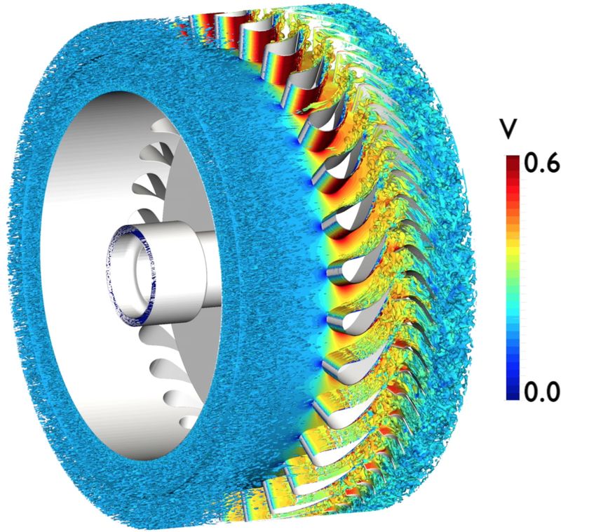
Joint hierarchical Cartesian mesh

       Hierarchical grid: parent-child relation between cells leads to tree structure
       Multiphysics method uses same tree structure for all physics
       Individual cells may be used for either physics1 , physics 2 , or both

                                                          l+3

                                                          l+2

                                                          l+1

                                                          l

5|29                                                                                    31st WSSP, March 16-19, 2021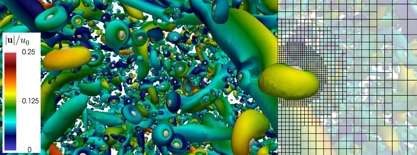
Domain decomposition using cell weights

                                                                              Hilbert curve
                lα

                lα + 1

                lα + 2

                lα + 3
                                   domain d                           domain d + 1

       Different cell weights ωx for physics 1 cells, physics 2 cells, or cells used for both
       Domain decomposition based on Hilbert curve
       Partitioning takes place at coarse level
       Complete subtrees distributed among ranks
 No MPI communication needed between all solvers

6|29                                                                                    31st WSSP, March 16-19, 2021
Parallel coupling algorithm
       Challenges for an efficient coupling algorithm
            Computational load composition varies between domains
            Solvers regularly need to exchange data internally
                                         time

                        domain       tCFD = tn            stage 1                         stage 2     tCFD = tn+1

                            0
                            1
                            2
                            3
                                    tCAA = tn−1                                                        tCAA = tn

                                                CFD computation              Start MPI communication (non-blocking)
                                                CAA computation              Finish MPI communication (blocking)

       Key components of the algorithm
           Both solvers composed of same number of “stages”
           Identical effort for each stage, only one communication step per stage
           Stages are interleaved for maximum efficiency
 Schlottke-Lakemper et al., Comput. Fluids, 2017
 Schlottke-Lakemper et al., Comput. Methods in Appl. Mech. Eng., 352, 2019
 Niemöller et al., Comput. Fluids, 2020
7|29                                                                                                           31st WSSP, March 16-19, 2021
Application: Particulate Flow

        Decaying isotropic turbulence, initial Reλ (t0 ) = 79
        E (k) = (3/2)u02 (k/kp2 )exp(−k/kp )
        up to 400,000 particles (spheres and ellipsoids) at dp ∼ η
 Schneiders, Günther, Meinke, Schröder. J. Comput. Phys. 311 (2016)
 Schneiders, Meinke, Schröder; J. Fluid Mech. 819 (2017)
 Schneiders, Fröhlich, Meinke, Schröder; J. Fluid Mech. 875 (2019)
8|29                                                                  31st WSSP, March 16-19, 2021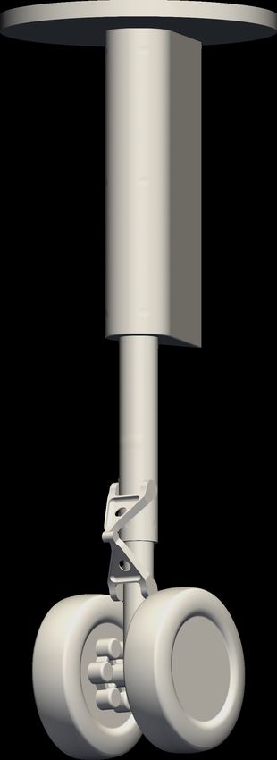
Motivation IC Engines

                         CO2 emissions: Gold Diesel vs. e-Golf

9|29                                                  31st WSSP, March 16-19, 2021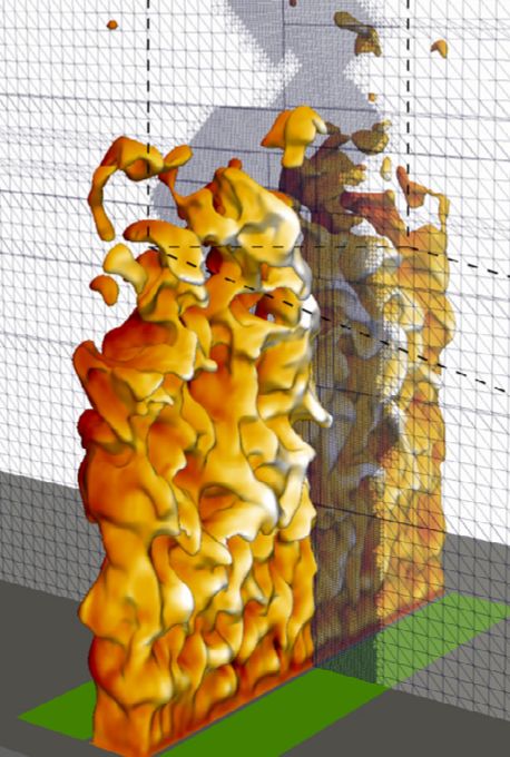
Motivation IC Engines

 Fuel Science Center (DFG funded Excellence Cluster @ RWTH)
    Biofuels allow realisation of a closed carbon
    cycle
    Green energy + bio material + CO2 ⇒ biofuels
    Advantages:
         established fuel distribution and engine
         technology can be used
         biofuels can be used as energy storage
Various potential biofuels exist such as Ethanol,
2-Butanone, Octanol, etc.
        Due to variations in thermo-physical properties
        targeted optimization is required
        Optimization and evaluation of novel engine
        concepts e.g. pre-chamber injection, multi-fuel
        injection
        Identify mixture-based criteria for optimal
        combustion
        Develop methods for automatic optimization
10|29                                                         31st WSSP, March 16-19, 2021
Fuel Mixing Simulation in IC Engines
Numerical method:
Perform large-eddy simulation of the flow field
Use a spray model for the injection of fuel
including evaporation and wall interaction
Cartesian mesh based finite volume solver for
the Navier-Stokes equation including species
equations
automatic solution for opening/closing of
valves by using a multiple level-set method
without the necessity of mesh topology changes
Spray model (4-way coupling)
Primary break-up modeled by multiple
injection points per timestep resulting in a
deterministic symmetrical hollow cone
2nd Break-up modelling: KHRT model
Dynamic load balancing for the time varying
domain size
Günther et al., "A flexible level-set approach for tracking multiple interacting interfaces in embedded boundary methods."
Comput. Fluids, 2014
11|29 31st WSSP, March 16-19, 2021Validation: IC Engine Spray Injection Simulation
Optical test engine Simulation Experiment
Bore 0.075 m
Stroke 0.0825 m
Compression 9.1:1
ratio
Valve lift 9 mm
Intake 0.1 MPa
pressure
Engine 1500 RPM
speed
PIV measurement setup
velocity magnitude (90o , 180o ATDC)
12|29 31st WSSP, March 16-19, 2021Validation: IC Engine Spray Injection Simulation
Turbulent kinetic energy k (includes CCV and
turbulent fluctuation)
engine-plane: whole engine cross-section
3 & 4-cycle: average across measurement Fuel spray validation experiment (top), simulation
window only (bottom)
13|29 31st WSSP, March 16-19, 2021Validation: IC Engine Spray Injection Simulation
Turbulent kinetic energy k (includes CCV and
turbulent fluctuation) Fuel spray validation for Ethanol and 2-Butanone
engine-plane: whole engine cross-section
3 & 4-cycle: average across measurement
window only
13|29 31st WSSP, March 16-19, 2021Ethanol and 2-Butanone Injection
Spray setup:
Injection for stochiometric conditions
Ethanol 40.7 mg (1.93 ms)
2-Butanone 34.9 mg (1.68 ms)
Computational setup:
Simulation on 1920 CPU cores of
HAWK@HLRS
Smallest spatial step 0.2 mm
maximum cell count 56 million
maximum number of parcels 7 million
(2-Butanone), 12 million (Ethanol)
Adaptive mesh refinement based on
surface location and droplet position
size of spheres indicates fuel parcel mass
in the volume 2 mm around the tumble plane
Ethanol 2-Butanone
concenctration at 100o and 110o ATDC
14|29 31st WSSP, March 16-19, 2021Results Ethanol and 2-Butanone Injection
volume ratio relative to stochiometric condition
liquid and evaoprated fuel volume
Ethanol 2-Butanone
15|29 31st WSSP, March 16-19, 2021Electrical Discharge Maschining (EDM)
Work piece is locally melted by sparks
generated by high voltage between electrode
and workpiece
Dielectric fluid in the working gap evaporates
and forms bubbles
Debris particles need to be removed to ensure
controlled discharge locations
Flushing flow is induced by electrode oscillation
or continuously establishing a flow
Allows accurate machining of extremely hard
material with small tolerances
Figure: Die-sink EDM process (WZL@RWTH)
16|29 31st WSSP, March 16-19, 2021EDM flushing flow
Efficient removal of debris particles and
gas is critical for the machining efficiency
Liquid-gaseous flushing flow
Density ratio ρl /ρg ≈ 1000
Viscosity ratio µl /µg ≈ 100
Gas volume fractions vary from 0 to 80 %
Debris transport
Large number of debris particles O(106 )
per flushing cycle
Figure: Pressure flushing EDM process (WZL@RWTH)
17|29 31st WSSP, March 16-19, 2021Numerical approach
gas
liquid
gas
High density/viscosity ratio and varying volume fractions → resolve each fluid phase separately
Ma < 0.1 → Lattice Boltzmann method for both fluid phases
Large number of small particles particles → Lagrangian particle tracking
Need for efficient surface reconstruction → Level set approach
Large number of degrees of freedom O(108 ) → Adaptive mesh refinement
18|29 31st WSSP, March 16-19, 2021Lattice Boltzmann method
Starting from the Boltzmann equation
Z Z
∂f ∂f Fi ∂f
ξ~r I ξ~r , Ω f 0 fβ0 − ffβ d Ωd ξ~β
+ ξi + =
∂t ∂xi m ∂ξi ξ~β Ω
following the BGK approach
∂f ∂f Fi ∂f
~ − f (ξ)
~
+ ξi + = ωc f eq (ξ)
∂t ∂xi m ∂ξi
and finally splitting the equation in two steps
~ t + δt ←
fi c ~x , ξ, ~ t + Ωc · f eq ~x , ξ,
fi ~x , ξ, ~ t − fi ~x , ξ,
~ t − 3wi gci · ez (1)
~ t + δt →
fi c ~x , ξ, fi p ~x + δt ξ~i , ξ,
~ t + δt (2)
19|29 31st WSSP, March 16-19, 2021Lattice Boltzmann Method
Using the incompressible equilibrium equation p20
p16
eq ci · ~u (ci · ~u )2 ~u 2 p7 p24
fi = wi (ρ + 2 + − )
cs 2cs4 2cs2 p10 p3
p21 p4 p9
the macroscopic flow variables can be recovered by
p0 p17 p12
27 27 p26 p25
p X X p18
ρ= = fi ~u = fi c i p11 p14 p1
cs2
i=1 i=1 p6 p5 p22
p2 p13
and
p19 p8
27 p15
1 X 1 ∂ui ∂uj
Sij = − (fi − fi eq )ci ⊗ ci = ( + ) y p23
2τ cs2 2 ∂xj ∂xi
i=1 z x
Figure: D3Q27 lattice definition
20|29 31st WSSP, March 16-19, 2021Multiphase Boundary condition
For each fluid (k = 1, 2), incoming
distributions are not set by propagation and
need to be determined separately Fluid 2
The macroscopic stress jump at the
boundary can be incoporated (Thömmes et al.
2009 )
(k) (k) ci · u~b 2wi 1
fi = fī +2wi − 2 Λi ((q− )S (k) +q(1−q)[S])
cs2 cs 2
1 [µ] Fluid 1
[S] : ~n ⊗ ~n = ([p] + 2σκ) − : ~n ⊗ ~n
2µ̄ µ̄
[µ]
[S] : ~n ⊗ ~tj = − : ~n ⊗ ~tj
µ̄ Figure: Missing distributions (2D)
21|29 31st WSSP, March 16-19, 2021Level set method
Signed distance function φ represents phase
boundary
Initialized by STL ray-tracing algorithm Fluid 2
Temporal change is described by transport φ=0
equation φ0
∇φ ∇φ
~n = κ=∇·
|∇φ| |∇φ|
Discretization ~n, κ
Spatial: Fifth-order upstream central Fluid 1
scheme
Temporal: Fifth-order Runge-Kutta
scheme Figure: Level set
High order constrained reinitialization to
preserve |∇φ| = 1 without changing φ0
22|29 31st WSSP, March 16-19, 2021Lagrangian Particle Tracking
Lagrange Particle Model
d~up ρ CD Rep
= (1 − ) · ~g + (~u − ~up ) (3)
dt ρp τp 24
ρ||~u − ~up ||2 dp ρp dp2 Fluid 2
Rep = τp = (4)
µ 18µ
Drag law
24 for Rep ≤ 0.1 u~p
Rep
2
24 1
CD = Re (1 + 6 Rep ) for Rep ≤ 1000
3 (5)
p
0.424 for Rep > 1000
Spatial interpolation of flow field to particle
position Fluid 1
High-order least-squares approach for
~u (~xp )
Low-order for ρ(~xp ) to capture density
discontinuity at interface
23|29 31st WSSP, March 16-19, 2021Joint hierarchical Cartesian mesh
gas
liquid
gas
Lattice Boltzmann Lattice Boltzmann
Level set Lagrange Particle
(liquid) (gas)
24|29 31st WSSP, March 16-19, 2021Joint hierarchical Cartesian mesh
LB (liquid) LB (gas) LS LPT
Hilbert
lα
curve
lα+1
lα+2
lα+3
domain domain
d d +1
Lagrangian Particle Tracking on hierarchical Cartesian grids
Domain decomposition based on Hilbert curve
Partitioning takes place at coarse level
Complete subtrees distributed among ranks
Each LPT cell stores the number of particles
No MPI communication needed between solvers
25|29 31st WSSP, March 16-19, 2021Rising bubbles in particle cloud
Figure: Three rising bubbles in a particle cloud at t/Tterminal = 0.2. Nparticle = 105 , Ngrid = 5 × 10⁶ .
ρl /ρg = 1000 µl /µg = 100 ρp /ρl = 7.7 Rel = 100 Eo = 5
26|29 31st WSSP, March 16-19, 2021Hawk Performance
Single node performance Fixed core count performance
Lattice Boltzmann solver (16 million cells) FV solver + combustion (18 species, 50000 cells)
strong scaling (1 Node) Varying core stride count (512 cores)
MPI parallelization MPI parallelization
10 1.2
ideal speedup
8 1 Node HAWK, LBM 1
1 Node AIA, LBM
speedup
6 0.8
speedup
0.6
4
0.4
2
0.2 HAWK, FV+Combustion
0 Claix, FV+Combustion
0
14
8
16
32
64
12
8
1
2
4
8
number of cores core stride count
Hawk: 2 x AMD EPYC 7742 (64 cores @ 2.25 GHz, AVX2)
CLAIX: 2 x Intel Xeon Platinum 8160 (24 cores @ 2.1 GHz)
AIA: 2 x Intel Xeon Gold 6148 (20 cores @ 2.4 GHz)
27|29 31st WSSP, March 16-19, 2021Hawk Hybrid OpenMP/MPI Parallelization
Lattice Boltzmann solver (80 million cells) Flow field around a landing gear
6 nodes (768 cores) (EU project Inventor)
Hybrid OpenMP/MPI parallelization
1.4 HAWK hybrid OpenMP/MPI
1.2
speedup
1
0.8
0.6
1
4
8
number of OpenMP Threads
preparatory study for the prediction of landing
gear noise
application of the coupled CFD + CAA solver
investigation of noise mitigation by porous
material
28|29 31st WSSP, March 16-19, 2021Summary
successful implementation of coupled multiphysics solvers for the analysis of engineering flow
prolems
hierarchical data structure is useful for the efficient parallelization
joint Cartesian mesh concept allows solution adaptive mesh with dynamic load balancing
large scale simulation runs are planned to be conducted on HAWK
Thanks to the HLRS staff for the continuous support!
Thanks for your attention!
29|29 31st WSSP, March 16-19, 2021You can also read