Ice microstructure and fabric: an up-to-date approach for measuring textures
←
→
Page content transcription
If your browser does not render page correctly, please read the page content below
Journal of Glaciology, Vol. 52, No. 179, 2006                                                                                 619

        Ice microstructure and fabric: an up-to-date approach for
                           measuring textures
               Gaël DURAND,1 O. GAGLIARDINI,2 Throstur THORSTEINSSON,3
                Anders SVENSSON,1 Sepp KIPFSTUHL,4 Dorthe DAHL-JENSEN1
               1
                 Ice and Climate Group, The Niels Bohr Institute, Rockefeller Complex, Juliane Maries Vej 30,
                                                DK-2100 Copenhagen, Denmark
                                                      E-mail: gd@gfy.ku.dk
           2
             Laboratoire de Glaciologie et Géophysique de l’Environnement (CNRS–UJF), 54 rue Moliere, `BP 96,
                                           38402 Saint-Martin-d’Hères Cedex, France
          3
            Institute of Earth Sciences, Building of Natural Sciences, Askja, Sturlugata 7, IS-101 Reykjavı́k, Iceland
        4
         Alfred Wegener Institute for Polar and Marine Research, Columbusstrasse, D-27568 Bremerhaven, Germany

           ABSTRACT. Automatic c-axes analyzers have been developed over the past few years, leading to a large
           improvement in the data available for analysis of ice crystal texture. Such an increase in the quality and
           quantity of data allows for stricter statistical estimates. The current textural parameters, i.e. fabric
           (crystallographic orientations) and microstructure (grain-boundary networks), are presented. These
           parameters define the state of the polycrystal and give information about the deformation undergone by
           the ice. To reflect the findings from automatic measurements, some parameter definitions are updated
           and new parameters are proposed. Moreover, a Matlab1 toolbox has been developed to extract all the
           textural parameters. This toolbox, which can be downloaded online, is briefly described.

1. INTRODUCTION                                                        It is worth noting that ice flow is strongly dependent on
                                                                   the texture. Firstly, the deformation of an ice crystal occurs
Ice cores provide a wonderful record to investigate past           by dislocation slip, mainly along the basal plane, confirming
climates. Since ice sheets form by successive deposition of        the predominant visco-plastic anisotropy of the ice crystal,
snow layers, travelling down to the deepest part of the ice        i.e. the resistance to shear on non-basal planes can be 60
sheet is a journey into the past. Ice-core studies provide a       times higher than resistance to shear along the basal planes
large set of climatic parameters, such as past temperature         (Duval and others, 1983). Due to the intrinsic anisotropy of
variations which can be revealed through isotopic data, the        ice, the c axes rotate during deformation towards compres-
atmospheric composition revealed through gas trapped in            sional axes and away from tensional axes (Azuma and
bubbles and the atmospheric circulation inferred from              Higashi, 1985; Castelnau and Duval, 1994; Van der Veen
impurity concentrations. Although there is an immense              and Whillans, 1994), and complex feedbacks occur
amount of information available, dating is the Achilles’           between flow and fabrics. As an example, under compres-
heel of these archives. For sites with high accumulation           sion, when c axes rotate toward the compressional axis, the
rates, counting of annual layers enables estimation of the         applied stress becomes increasingly perpendicular to the
age (Greenland Icecore Project (GRIP), Greenland Ice               basal plane, and the ice becomes harder to compress.
Sheet Project 2 (GISP2) and NorthGRIP cores among                  Secondly, the rheology may depend on the mean crystal
others; see, e.g., Alley and others, 1997b). At depths where       size, as finer grains could explain a third of the shear strain
annual layers are not resolvable, and for sites with low           rate enhancement observed in ice deposited during glacial
accumulation rates, flow models have to be used to                 periods (Cuffey and others, 2000). Understanding the
reconstruct the sinking of the ice layers and then the age         reasons for grain-size variations with climatic changes is
can be estimated with depth (Dome C, Vostok and Dome F             thus an important task for texture studies (Durand and
(Antarctica) cores among others; see, e.g., Parrenin and           others, 2006). Finally, recrystallization processes have to be
others, 2001). Consequently, understanding the deform-             taken into account. As an example, rotation recrystalliza-
ation of the ice is of primary importance for correct              tion, also known as polygonization, is characterized by
climatic interpretation.                                           basal dislocations that group together in walls perpendicular
   From a material science point of view, ice is an                to the basal planes and form sub-boundaries. The misor-
assemblage of crystals with a hexagonal crystallographic           ientation between two subgrains increases gradually, and
structure. The crystal orientation is specified by the direction   grains may split into smaller grains. Such processes
of its a and c axes. Due to the birefringence of ice, the c axis   complicate the interpretation of texture measurements.
of a single crystal, which is perpendicular to the basal               Since the texture records the deformation history of the
planes, can be easily revealed by optical measurements. In         ice, an understanding of processes affecting the texture may
what follows, ‘fabric’ refers to the orientations of the c axes    lead to a better understanding of ice flow. Moreover, the
of the ice polycrystal, whereas ‘microstructure’ refers to the     complex feedbacks between fabric development and de-
grain-boundary network. The term texture includes both the         formation are now incorporated in local flow modelling
fabric and microstructure. Note that this terminology is not       (Gagliardini and Meyssonnier, 2000). In such models, both
universally accepted, and other usages of these terms can be       the velocity and the fabric fields are calculated, allowing
found in the literature.                                           comparison with measurements. Such comparisons require
620                                                                                 Durand and others: Ice microstructure and fabric

some fabric parameters that can be determined both                   the quality of the thin section: melting more than
theoretically and experimentally. Last but not least, in some        necessary can induce bubble trapping at the glass–ice
cases, the study of the texture can help to explain observed         interface; conversely, too little heat applied to the glass
flow disturbances such as folds (Alley and others, 1997a;            plate will cause a weak bond between ice and glass and
Raynaud and others, 2005). This is crucial for extracting            the thin section may be damaged while reducing the
palaeoclimatic records from an ice core.                             thickness. This method needs practice before satisfactory
   Due to the birefringence of ice crystals, ice texture can be      results can be obtained. The sample can also be fixed by
revealed by the examination of a thin section under cross-           using water droplets on its border as in step 2. This
polarized light. Earlier studies of ice texture were made            procedure is easier than that proposed by Langway
manually, which was tedious and particularly time-consum-            (1958), and the quality of the final thin section is
ing work. Much progress has been made in developing ice-             generally better.
texture instruments, and now automatic measurements of
                                                                  4. Using a bandsaw, the sample is cut parallel to the glass
texture can be performed. Wilen and others (2003)
                                                                     plate, leaving 1–2 mm of ice adhering to the glass.
presented a review of the automatic ice-fabric analyzers
(AIFAs) used in the glaciological community. In the cited         5. The section is reduced to a thickness of 0.3 mm with a
works, the AIFAs were mainly used to extract the grain               microtome knife. The thickness is an important par-
orientations of an ice sample, and microstructure was                ameter for grain-boundary determination using cross-
considered as a by-product of the measurements.                      polarized light. Sharp colour transitions between grains
   As plentiful and more robust measurements have now                are required and interference fringes, which appear if the
been obtained using an automatic ice-texture analyzer                grain boundary is too thick, should be avoided. The
(AITA; since one should also extract the microstructure of           optimal thickness corresponds to grain colour in the
a sample using an AIFA, AITA is a more appropriate term),            brown–yellow range (Gay and Weiss, 1999).
some of the textural parameters measured so far are, in our
                                                                  It is obvious that the measurements result from two-
view, now obsolete. Moreover, new parameters can be
                                                                  dimensional (2-D) cuts of a three-dimensional (3-D)
defined. These parameters better describe the texture and
                                                                  structure. This point, referred to as the sectioning effect in
should be used in preference to earlier ones. This paper aims
                                                                  what follows, must always be kept in mind, as it influences
to review and propose new methods to describe ice texture.
                                                                  the interpretation of the measurements made on the
The paper is organized as follows: in section 2, we discuss in
                                                                  microstructure (see Underwood (1970) for a review of
detail the operations needed to obtain the texture informa-
                                                                  stereological problems, and section 3.1.2 for a discussion of
tion from an ice sample. In section 3, we review the
                                                                  the influence of 2-D cuts on mean grain radius estimation).
parameters used so far to describe the microstructure and
                                                                  The c-axis measurement is not influenced by this 2-D effect,
propose new definitions. Section 4 deals with fabric
                                                                  assuming a small disorientation within a grain.
parameters. Finally, section 5 briefly presents a Matlab1
tool to determine all these texture parameters.                   2.2. Texture measurements
                                                                  The classical manual technique for measuring the fabric of a
2. MEASUREMENTS                                                   thin section is based on the Rigsby-stage procedure (Rigsby,
                                                                  1951) that was standardized by Langway (1958). Micro-
2.1. Sample preparation                                           structural parameters, such as the mean grain size, were also
Most of the studies of ice texture follow the standard            estimated manually (see section 3.1). More recently, image-
procedure detailed in Langway (1958) to prepare thin              analysis procedures have allowed extraction of microstruc-
sections. Here, we briefly recall this procedure and propose      ture and new parameters related to the shape of grains (Gay
some improvements:                                                and Weiss, 1999; Svensson and others, 2003).
1. A vertical (parallel to the core axis) or a horizontal            Today, using an AITA, the whole texture of a polycrystal
   (perpendicular to the core axis) thick section about 1 cm      can be measured: fabric and microstructural parameters can
   thick is cut from the ice core. The sample location differs    now be obtained together on the same sample. Indeed,
   from core to core, but a large sample area is preferable       Gagliardini and others (2004) have shown that the measured
   (this point is detailed later).                                cross-sectional area should be used as a statistical weight of
                                                                  the polycrystal constituents in order to improve the fabric
2. One surface of the sample has to be flattened in order to      description. Complete texture measurements are also
   obtain a plane surface. As proposed by Langway (1958),         pertinent, as mapping of the spatial distribution of c axes
   sandpaper can be used, but Thorsteinsson (1996)                can reveal additional information about recrystallization
   proposed another procedure: The thick section is placed        processes (Alley and others, 1995; see also section 4.7).
   on a glass plate, with a few drops of water along its side        Two major steps have to be carried out to extract the
   to glue it to the glass plate. The plate is fixed to a         texture from the output of an AITA:
   microtome and is shaved to produce a smooth and plane
                                                                  1. Extraction of grain boundaries. Gay and Weiss (1999)
   surface. Then the sample is removed from the glass plate
                                                                     proposed an image analysis algorithm to extract the
   by breaking the frozen-water droplets with a cutter. In
                                                                     microstructure from three images of one thin section
   our experience, the second procedure is preferable as it
                                                                     taken under cross-polarized light. After some filtering to
   produces better results.
                                                                     remove noise, a Sobel filter is used to detect large
3. A glass plate is then frozen or glued onto the smooth             discontinuities in intensity, which generally correspond
   surface. Langway (1958) proposed the glass plate be               to grain boundaries. This method works well for
   warmed and the sample glued by refreezing of water. The           randomly oriented crystals, as the colour variations from
   amount of heat applied to the glass plate will determine          grain to grain are important (see Fig. 1). For more
Durand and others: Ice microstructure and fabric 621
oriented fabrics, colours between grains are similar and
grain-boundary detection is more difficult and some
manual corrections are needed. Note also that the
resulting microstructure is naturally strongly dependent
on the quality of the thin section. Most of the existing
automatic machines produce images of the thin sections
that can be used to extract the microstructure (Wilen and
others, 2003). An adaptation of the Gay and Weiss
(1999) algorithm can easily be made from the output of
these analyzers.
2. Assigning an orientation for each grain detected in (1). Fig. 1. Image of a thin section under cross-polarized light (left) and
Using an AITA, the orientation is known for each pixel of the corresponding texture (right). Grain boundaries appear white,
the grain. The initial measurements for a given pixel are and each grain defined within the microstructure has an orientation
the co-latitude, p , and the longitude, ’p , if this pixel is detailed in the colour map given by the polar plot projection shown
not located on a grain boundary. An average value of the on the bottom right.
c axis over all pixels inside a grain, as well as the
dispersion, can be estimated within each grain. These
calculations are detailed in section 4.5. Thorsteinsson and others (1997) estimated the mean grain
Finally, from outputs of the AITA, one obtains the complete size along the GRIP core using the linear intercept method.
description of the texture at the grain scale. That is the This method consists of counting the number of grain
microstructure, which contains all the topological informa- boundaries that intercept a horizontal (or vertical) line. This
tion, and the fabric which gives the mean orientation of all leads to the estimate of a mean intercept length, hLi, which
non-intersecting grains within the microstructure. Such for a regular surface is proportional to the square root of the
results allow the construction of images such as that shown area of the considered object (Underwood, 1970). This
in Figure 1, which contain all the information required to method suffers different biases: (1) if the grain shape evolves
calculate the parameters describing the texture (see sections (and that is the case; see Durand and others, 2004), the ratio
3 and 4). It is worth noting that the original outputs from the between the mean area and hLi is affected; (2) twisted grain
AITA should be conserved, as they certainly contain boundaries can intercept a given line more than once; and
information at the sub-grain scale that is not taken into (3) the link between the grain-area distribution and the
account in this work and may be useful at a later date. distribution of the length of intercept is not straightforward.
Duval and Lorius (1980) estimated the mean grain area by
counting the number of grains within a defined surface. As
3. MICROSTRUCTURAL PARAMETERS this method takes into account the whole population of
grains, it is more robust than the method proposed by Gow
Manual estimation of the grain size is time-consuming work (1969). It also provides a more straightforward estimate of
and several methods have been used so far to make these the mean grain size than the linear intercept method, but it
measurements practicable. As discussed in section 2, image- does not provide a grain-size distribution. Note also that
analysis procedures now provide the ability to extract the corrections are required in ice with significant porosity.
complete microstructure in an acceptable time. Therefore, a
more accurate definition of the grain size can be made, and 3.1.2. Mean grain radius
the procedures also give new information on grain-size A more complete way to measure a characteristic length of
distributions. Comparisons of the different methods used so the microstructure would be to calculate the average
far are reviewed in section 3.1. PNg 1=3
Other studies have focused on the grain shape to obtain volumetric radius: hRV i ¼ 1=Ng k¼1 Vk , where Ng is
information about ice deformation (Azuma and others, the number of non-intersecting grains within the micro-
2000; Durand and others, 2004). As for the measurement structure and Vk is the volume of grain k. As mentioned
of the grain size, several methods have been used so far; a previously, the volume of the ice crystal cannot be measured
comparison is provided in section 3.2. and 2-D sections have to be made. Then a characteristic
length of the microstructure could be expressed by the
3.1. Grain size average radius:
3.1.1. Estimation of a characteristic length of the
1 X 1=2
Ng
microstructure hRi ¼ A , ð1Þ
Gow (1969) first proposed measuring the mean grain size of Ng k¼1 k
a section by estimating the average area of the 50 largest
grains. By definition, this method only measures the where Ak is the cross-sectional area of grain k and
evolution of the largest part of the grain distribution; thus, Ak ¼ Npk , where is the actual area of a pixel and Npk is
it is not representative of the complete population. It is also the number of pixels that compose grain k. An estimate of
worth noting that the representativity of the 50 largest grains the error induced by the sectioning effect can be made with
is affected by a change in the grain size (for a constant the help of a 3-D Potts model. In such a model, 3-D
sampling surface). This leads to a bias in the estimation of microstructure is divided into small volume elements and an
grain-growth rate (Gay and Weiss, 1999). The method was orientation is allocated to each element. Grain growth is
developed in order to perform manual measurements and simulated using a Monte Carlo technique: an element is
should be avoided for automatic measurements. randomly selected and a new orientation is randomly622 Durand and others: Ice microstructure and fabric
Fig. 3. Evolution of the standard deviation of hRi over hRRef i vs the
Fig. 2. Normalized distribution of the logarithm of the normalized inverse of the square root of the number of grains.
radius of the grain (Rk =hRi) for a microstructure sampled along the
EPICA Dome C (Antarctica) core at 100.1 m depth (black line). The
log-normal distribution corresponding to the measured parameters
hiD and D of this microstructure is also plotted (dotted line), as well
as the distribution obtained for a 2-D Potts microstructure (grey
line). The number of grains (275) and the mean radius (21.3 pixels)
of the Potts microstructure are comparable to the natural sample that these microstructures present enough grains to com-
(454 grains and hRi ¼ 21:6 pixels). pletely describe the grain-size distribution. Their mean
radius was then used as a reference, hRRef i. For each
microstructure, 80 subsampling microstructures were ran-
domly selected. These sub-microstructures contained be-
attributed. Similar orientations between neighbouring ele- tween 3 and 200 grains and their mean radius was
ments (i.e. same grain) will decrease the energy of the calculated and compared to hRi. As hRi=hRRef i follows the
system, and the new orientation will then be conserved. The central limit theorem, the standard deviation depends only
Potts model is known to properly reproduce the topological, on the number of grains, following the relation
kinetic, grain-size distribution and morphological features of 1=2
p ðhRi=hRRef iÞ ¼ 0:44Ng (see Fig. 3). Of course, for
normal grain growth (Anderson and others, 1989), such as
measurements on natural ice, hRRef i is unknown, and we
recrystallization processes occurring in the upper part of ice
make the following approximation:
sheets (Alley and others, 1986).
Following Gagliardini and others (2004), we generated p ðhRiÞ ¼ p ðhRi=hRRef iÞhRRef i p ðhRi=hRRef iÞhRi ð2Þ
3-D Potts microstructures containing 400 400 400 ele-
1=2
ments. A section within this volume contains approximately and finally obtain p 0:44Ng hRi. An error bar that
200 non-intersecting grains. For such a section, both hRV i takes into account the sectioning effect (s ) as well as the
and hRi can be measured and compared. From these results, population effect (p ) can now be attached to hRi as follows:
we demonstrated that the standard deviation s of the hRi
distribution for a given hRV i can be approximated by ðhRiÞ ¼ s þ p 0:02 þ 0:44Ng1=2 hRi , ð3Þ
s 0:02hRi (Durand, 2004).
The mean grain size generally increases with depth Alley where hRi is calculated using Equation (1).
and others, 1986), and for a constant sampling surface the
number of grains will decrease with increasing depth. The 3.1.3. Distribution parameters
statistics for the calculation of the average grain radius can Under normal grain growth, the normalized grain-size
be drastically affected. As for the error induced by the distribution, Rk =hRi, remains unchanged and is closely
sectioning effect, we estimate the error induced by the approximated by a log-normal distribution (Humphreys and
number of grains used in the calculation of the average Hatherly, 1996). This observation does not have a theoretical
radius using a Potts model. Anderson and others (1989) have explanation as yet; it is, however, a useful description, as the
shown that a 2-D Potts model reproduces the characteristics distribution can be completely defined with only two, easily
of a microstructure determined from a section of a 3-D measurable, parameters: the mean, hiD ¼ hlnðRk =hRiÞi , and
polycrystal under normal grain growth (and the calculation the standard deviation, D ¼ ½ ln ðRk =hRiÞ. Changes in the
time is much smaller for 2-D than for 3-D simulations). As normalized distribution could reveal changes in the
shown in Figure 2, the normalized grain-size distribution of activated recrystallization processes. Such changes could
a 2-D Potts microstructure is highly comparable with a also provide information on the mechanisms affecting the
natural microstructure sampled along the EPICA (European normal grain growth, such as pinning of grain boundaries by
Project for Ice Coring in Antarctica) Dome C core (75806’ S, microparticles which induces a shift of hiD and D (Riege
123821’ E) at 100.1 m depth (see also section 3.1.3). and others, 1998; Durand and others, 2006).
We simulated 200 microstructures of 10002 pixels From Potts model results, and following the procedure
containing between 622 and 1808 grains. We supposed detailed in section 3.1.2, we also estimate the intrinsicDurand and others: Ice microstructure and fabric 623
variability of hiD and D induced by the sectioning effect and examined under different scales: a small p explores
the change in the population: details, whereas a larger p improves the statistics.
Compared to the inertia tensor presented in Equa-
ðhiD Þ ¼ 0:06 þ 1:83 Ng1=2 hiD tion (2), M has the additional advantage that it has a
physical significance in terms of mechanical deformation
ðD Þ ¼ 0:04 þ 0:95 Ng1=2 D : (Aubouy and others, 2003). From the variation of M with
respect to a reference M0, a statistical strain tensor, U,
3.2. Grain shape and deformation of the which coincides with the classical definition of strain
microstructure (Aubouy and others, 2003), can be defined. As M0
cannot be measured for natural ice, Durand and others
Many different descriptors can be used to determine the (2004) assume that the deformation is isochoric, and that
shape of grains and quantify the anisotropy of a micro- the reference state is isotropic, leading to the following
structure (Mecke and Stoyan, 2002). Many have been expression:
applied by the glaciological community, so comparison 0 1
1
between different results from different cores can sometimes 1 @ log 2 0
be tricky. Among the most frequently used parameters are: U¼ R AR 1 : ð5Þ
4 0 log 21
1. Comparison between the mean vertical and horizontal
intercept lengths (Thorsteinsson and others, 1997; Gay Note that some statistical tests, comparable to those
and Weiss, 1999). In addition to the inherent artefacts presented in section 3.1.2, have been carried out to
induced by the measurement of hLi (see section 3.1.1), estimate the intrinsic variability of U that leads to
this method is not able to correctly quantify anisotropy in ðU Þ ¼ 0:35N 1=2 (Durand and others, 2004).
a non-horizontal plane. A similar method was used by Note that Durand and others (2004) called M the texture
Svensson and others (2003), as they measured the tensor and used different notation. To avoid confusion with
bounding box of each grain and calculated the corres- our definition of texture (see section 1), M will be denoted
ponding aspect ratio, i.e. the width-to-height ratio of the the microstructure anisotropy tensor.
smallest rectangle with horizontal and vertical sides
which completely encloses the grain. Such a method also
does not fully capture grain elongation that is not 4. FABRIC PARAMETERS
oriented in the horizontal or vertical directions, unless
This section presents some tools that allow description of the
the box orientations are rotated.
fabric measured from a thin section containing Ng non-
2. An inertia tensor for each grain can also be calculated intersecting crystals. In this section each individual crystal is
(Azuma and others, 2000; Wilen and others, 2003). The described by:
eigenvalues of the tensor provide the elongation of the
grain, and the eigenvectors give the directions of 1. Its orientation c k . The orientation of the ice crystal is
elongations. Compared to the previous methods, this described by its c-axis orientation, which is defined by
tensor description has the advantage that the obtained two angles: the co-latitude k 2 ½0, =2 (or tilt angle) and
measurements do not depend on the particular choice of the longitude ’k 2 ½0, 2 given in the local reference
axes (e.g. vertical and horizontal). frame, R, which has its e3 axis perpendicular to the thin
section. The expression of c k in this reference frame is
3. Durand and others (2004) proposed a new method based
on the vectors, ‘, that link neighbouring triple-junction c k ¼ ðcos ’k sin k , sin ’k sin k , cos k Þ: ð6Þ
locations (where three grain boundaries meet). This
method, which can suffer from some artefacts in porous 2. Its volume-weighted fraction, fk . Larger crystals should
ice (triple junctions may occur in pores), is briefly have more influence on the polycrystal behaviour than
recalled here. More details and applications can be smaller ones. As suggested by Gagliardini and others
found in Durand and others (2004). A local average (2004), to estimate the volume of grain k from 2-D thin-
microstructure anisotropy tensor, M, can be defined as: section measurements, one can assume that it is
* !+ proportional to its measured cross-sectional area, Ak .
‘21 ‘1 ‘2 Then, the volume-weighted fraction is:
M¼
‘2 ‘1 ‘22 3=2
p A
fk ¼ PNg k : ð7Þ
1 X N
Aj
3=2
¼ ‘ðjÞ ‘ðjÞ j¼1
N k¼1
In what follows, the fabric of the polycrystal is given in
1 0 terms of the distribution of the Ng c-axis orientations, c k ,
¼R R 1 , ð4Þ
0 2 and the Ng weight fractions, fk .
where ð‘1 , ‘2 Þ are the coordinates of ‘ in the local
reference frame, R, (the e3 axis is perpendicular to the 4.1. Rotation of reference frame and polar
thin section). The absolute horizontal orientation is representations
unknown; e1 is relative to the thin section, which cannot 4.1.1. Rotation of reference frame
be oriented with respect to the core axis. R is the rotation Most studies of ice fabrics use equal-area point plots (also
which makes M diagonal and ð1 , 2 Þ are the corres- named Schmidt point plots) to present the distribution of c k
ponding eigenvalues; hip denotes the average over N axes in a thin section (e.g. Thorsteinsson and others, 1997;
vectors, up to the pth neighbours. A sample can be see also Fig. 4a). In the literature, the polar plots are624 Durand and others: Ice microstructure and fabric
underlying large population of crystals. The data are then
^
used to create a robust estimate, GðxÞ, of GðxÞ. With Ng
data points, GðxÞ is represented as a superposition of Ng
simpler normal probability-density distributions, gk ðxÞ, for
Ng sub-populations,
X
Ng
GðxÞ ¼ fk gk ðxÞ: ð11Þ
k¼1
GðxÞ is then projected onto an equal-area diagram using
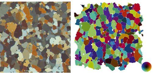
Fig. 4. Point plots (a) and contour plots (b) of the inferred
probability-density distributions of the fabric at 2999.8 m depth in
Equation (10) to produce Gðx, yÞ.
the Dome C ice core. The probability-density distribution, G, is For each crystal orientation, c k , the orientation-
contoured at levels of ¼ 1=ð6Þ. distribution density of the associated kth sub-population
on a hemisphere centered on axis c k is defined as:
1
gk ðxÞ ¼ exp 2 x c x c
k k
, ð12Þ
22 2
represented in a horizontal reference frame, R h , i.e. the in
where is a normalizing factor to account for the spread of
situ vertical (the core axis) is at the centre of the polar plot
the Gaussian on a hemisphere. In practice, ’ 1 if there are
(Langway, 1958). Therefore, if thin sections are cut vertically,
ten or more crystals to contour.
the fabrics need to be rotated for easier comparison of fabric
diagrams. To obtain a horizontal projection from a vertical Each gk ðxÞ has a mean orientation given by c k, and the
width of the component normal probability-density distri-
thin section, one needs to rotate c k as follows:
bution is ¼ M þ N , where M is the spread due to
’hk ¼ arctanðtan vk sin ’vk Þ 2 ½0, 2 measurement error, and N represents spread due to limited
hk ¼ arccosðsin vk cos ’vk Þ 2 ½0, =2 ð8Þ sample size, Ng . Using numerical experiments, it can be
shown that the ‘best’ (for 40 or more crystals) is
pffiffiffiffiffiffi
where ’hk and hk are the longitude and co-latitude in the ¼2 Ng .
horizontal reference frame, and ’vk and vk are those in the The expected value of GðxÞ for isotropic ice is
vertical frame. In this horizontal reference frame R h ; the e3h E ¼ 1=ð2Þ, and real clusters should exceed the
axis points vertically upward. If the thin section is cut E þ 1=ð3Þ contours, that is E 2, where ¼ 1=ð6Þ.
horizontally R ¼ R h. The function G should be contoured at 2, 4, . . . intervals,
with larger spacing if very strong maxima occur. A
4.1.2. Equal-area (Schmidt) point plots and contoured comparison between a classical point plot and a contoured
data plots data plot is presented in Figure 4 for a Dome C texture
The equal-area projection (Kocks, 1998, p. 54) is achieved sampled at 2999.8 m depth. The contour plot with Ng ¼ 80
by the coordinate transformation: illustrates very clearly the strength of the clustering of
crystals near the vertical. Such an observation is less obvious
hk in the point plot. More details will be given in a forth-
¼ 2 sin , ð9Þ
2 coming paper.
and
4.2. Strength of fabric and spherical aperture
xk ¼ cos ’hk , yk ¼ sin ’hk : ð10Þ The strength of fabric (also called degree of orientation or
This transformation takes all points in the upper hemisphere strength of orientation) is a one-parameter fabric descriptor
pffiffiffi that has been widely used in the glaciology community. This
and projects them within a circle of radius 2 on the x-y
plane. An equal-area point plot then simply puts a marker at is mainly because most of the observed ice fabrics are one-
the ðxk , yk Þ location of each crystal orientation. maximum or girdle-type fabrics and therefore present a
The purpose of presenting c-axis distributions is often to symmetry axis.
learn as much as possible about the fabric in nearby ice, The definition of the strength of fabric that can be found
not merely to present a specific dataset (Kamb, 1959). in the literature (Thorsteinsson and others, 1997; Castelnau
Now that data are collected using automatic methods and others, 1998; Gagliardini and Meyssonnier, 2000) is:
(Wilen, 2000), a collection of several hundred to over a X
Ng
thousand measured crystal orientations is common. This Rs ¼ 2 fk c k 1 , ð13Þ
results in the problem of overlapping points when k¼1
presenting the data on point plots. Some authors (Langway, where jj:jj is the norm of a vector. This definition of the
1958; Kamb, 1959) have presented fabric information strength of fabric assumes implicitly that the fabric has a
using contour plots. symmetry axis and that this symmetry axis is the axis e3
Because any sample is limited in its size, Ng , we can, at perpendicular to the thin section. Therefore, this parameter
best, get an imperfect estimate of the underlying popula- is not objective since it depends on the reference frame
tion. Estimates that are robust are desirable. A new where the sum is performed.
approach, which stems largely from Kamb (1959) is A more rigorous definition, but still not objective, for the
currently under development and is briefly described here. strength of fabric, Rs , needs to first calculate the ‘best’
It is first assumed that there is an unknown ‘global’ symmetry axis for the fabric. Later we will present two
^
orientation probability-density distribution, GðxÞ, for the different methods to effectively determine this fabricDurand and others: Ice microstructure and fabric 625
symmetry axis, c . Here, assuming that c is known, the that, despite the historical point of view and comparisons
strength-of-fabric parameter is calculated as: with old datasets, there is no longer a reason to use these
two parameters. As shown below, the second-order orien-
X
Ng
Rs ¼ 2 c c k Þc k 1:
fk signð ð14Þ tation tensor contains much more information and should be
k¼1 preferred.
The sign operator allows us to perform the sum within the 4.4. Orientation tensors
hemisphere centred on the fabric symmetry axis, c. Never-
4.4.1. Second-order orientation tensor
theless, with this new definition, the same problem still
As suggested by Woodcock (1977), a good way to
occurs for the grains which have their c axis perpendicular
characterize the essential features of an orientation distri-
to
c, for which c c k ¼ 0 and no sign can be determined.
bution is to use the second-order orientation tensor, að2Þ ,
Note that, as mentioned previously, Equations (14) and (13)
defined as:
are equivalent only if c¼ e3 .
The spherical aperture, s , is directly related to the X
Ng
strength of fabric by: að2Þ ¼ fk c k c k , ð18Þ
pffiffiffiffiffiffiffiffiffiffiffiffiffi k¼1
s ¼ arcsin 1 Rs : ð15Þ
For isotropic ice Rs ¼ 0 and s ¼ 90 and for a single- where c k is given by Equation (6) and fk by Equation (7). By
maximum fabric Rs¼1 and s ¼ 0 . For fabrics with girdle construction, að2Þ is symmetric and there exists a symmetry
tendency, 1 R < 0 and, due to its definition, s is reference frame, Rsym (or principal reference frame), in
ð2Þ
unusable. which að2Þ is diagonal. Let ai (i = 1,2,3) denote the three
corresponding eigenvalues and o e i (i = 1,2,3) the associated
4.3. ‘Best’ symmetry axis of a fabric eigenvectors, which correspond to the three base vectors of
A first method to calculate the ‘best’ symmetry axis of a Rsym. The eigenvalues of að2Þ can be seen as the lengths of
fabric is to use a least-squares method to minimize the sum the axes of the ellipsoid that best fit the density distribution
of the squared angle between the symmetry axis and all the c of the grain orientations. The eigenvectors then give the axis
axes, c k . That is, we need to find
c which minimizes: directions of this ellipsoid.
ð2Þ ð2Þ ð2Þ
X
Ng The three eigenvalues a1 , a2 and a3 follow the
2 ¼
fk 2k , ð16Þ relations:
k¼1
ð2Þ ð2Þ ð2Þ
where k is the angle between
c and c k : a1 þ a2 þ a3 ¼ 1 ð19Þ
cos k ¼ j
c ck j ð17Þ ð2Þ ð2Þ ð2Þ
0 a3 a2 a1 1: ð20Þ
(assuming c is a unit vector). ð2Þ ð2Þ ð2Þ
The absolute value in Equation (17) is to take into account For an isotropic fabric, a1 ¼ a2 ¼ a3 ¼ 1=3, and when
that each vector c k must be in the same hemisphere as c. the fabric is transversely isotropic, two of the eigenvalues are
The minimum value of depends on the fabric type. For a equal:
pffiffiffiffiffiffiffiffiffiffiffiffi
¼ 2 61 and for a single-
perfectly isotropic fabric ð2Þ ð2Þ
pffiffiffiffiffiffiffiffiffiffiffiffi a2 a3 < 1=3 for a single-maximum fabric,
maximum-type fabric 2 > 0, whereas for a girdle-
pffiffiffiffiffiffiffiffiffiffiffiffi ð2Þ
ð2Þ
> 1=3 ð21Þ
type fabric =2 > 2. Due to the absolute value, a1 a2 for a girdle fabric:
this problem is not continuous and may present some local
According to Woodcock (1977), fabrics that have equal
minima. ð2Þ ð2Þ
A second solution is to define the symmetry axis, c, as the girdle and cluster tendencies are such that a1 =a2 ¼
ð2Þ ð2Þ
first eigenvector obtained from the calculation of the a2 =a3 . Then, the use of the parameter
eigenvalues of the second-order orientation tensor, as . . .
ð2Þ ð2Þ ð2Þ ð2Þ
presented below. This tensor is obtained from the direct ¼ ln a1 a2 ln a2 a3
calculation of the average of the dyadic product of the
c axes. By definition, there is no ambiguity from the c-axes gives objective information about the fabric shape: > 1
orientations for the calculation of the second-order orien- for single-maximum fabric and < 1 for girdle-type
tation tensor. fabric. As suggested by Woodcock (1977), one should use
.
The difference in
c resulting from these two methods can ð2Þ ð2Þ
C ¼ ln a1 a3 as a measure of the strength of the
be large, especially when the fabric is not concentrated. As
an example, for a randomly distributed fabric, the angle preferred orientation. C varies from 0 for randomly distrib-
between the c obtained by the two different methods can be uted orientations to infinity when all the orientations are
up to 308. This is because for a perfectly randomly distributed identical.
fabric there are an infinite number of ‘best’ symmetry axes, c The three eigenvectors, o e i , define the ‘best’ material
(every axis is a symmetry axis for such a fabric). symmetry reference frame of the sample. It is often useful to
In what follows, the ‘best’ symmetry axis is determined calculate the angle between the main symmetry axis of the
using the second method. Moreover, since both the strength fabric, o e i , and the local vertical:
of fabric, Rs , and the spherical aperture, s , require
knowledge of the mean symmetry axis of the grain ¼ arccos o e 1 e h3 2 ½0, =2 , ð22Þ
orientations and, consequently, calculation of the eigen-
vectors of the second-order orientation tensor, we believe where the e hi are the basis vectors of R h .626 Durand and others: Ice microstructure and fabric
The study of higher-order orientation tensors allows orientation tensors to describe fabrics, as was mentioned
investigation of the gap between the actual fabric and the above, for the strength of fabric, Rs , or the spherical
orthotropic fabric constructed by the use of the second-order aperture, s .
orientation tensor.
4.5. Average and dispersion of the c axes within
4.4.2. Higher-order orientation tensors a grain
By definition, the fourth-order orientation tensor is: Using an AITA, the initial measurement gives the orientation
X
Ng of each pixel in the sample. After extraction of the
að4Þ ¼ fk c k c k c k c k : ð23Þ microstructure, one has to determine the mean orientation,
k¼1 c k , for each grain, as used in the previous sections. As for a
The fourth-order orientation tensor contains more informa- grain, Equation (6) applies for the pixel orientation vector.
tion about the fabric than the second-order orientation Since, similarly to a grain, a pixel can be oriented by
tensor and can reproduce non-orthotropic fabric. If the either c p or c p, the mean orientation of a grain, c k , cannot
fabric is orthotropic then, by construction, the fourth-order be calculated as the average value over the Npk orientations
orientation tensor has the same principal axis as the second- c p . As for the whole thin section, the mean orientation of the
order one, and only 21 of its 81 components are non-nulls grain has to be determined as the first eigenvector of the
when expressed in the symmetry reference frame R sym . second-order orientation tensor calculated on the grain, i.e.
Moreover, according to Cintra and Tucker (1995) only 3 of for a given grain k, c k ¼ o e k1 , where o e k1 is the first
these 21 components are independent. The 21 non-null eigenvector of the second-order orientation tensor defined
components are:
by Equation (18) in which Ng has been replaced by Npk.
ð4Þ ð4Þ ð4Þ
af1122g , af1133g , af2233g , Contrary to a polycrystalline fabric, adjacent pixel
ð4Þ ð2Þ ð4Þ ð4Þ orientations on the same grain should be very close except
a1111 ¼ a11 a1122 a1133 , when crossing a subgrain. Nevertheless, some artefacts are
ð4Þ ð2Þ ð4Þ ð4Þ still present for some pixels and these pixels need to be
a2222 ¼ a22 a2211 a2233 ,
excluded from further calculations. Indeed, for a given view,
ð4Þ ð2Þ ð4Þ ð4Þ
a3333 ¼ a33 a3311 a3322 , ð24Þ the determination of the extinction angle constrains c p to lie
along two orthogonal planes. The AITAs repeat the measure-
where aiijj denotes the series of components independent of
ments for three different views that should unambiguously
the order of the indices aiijj ¼ aijij ¼ aijji ¼ ajiij ¼ ajiji ¼ ajjii . determine c p . Unfortunately, for some pixels the extinction
The 60 other components are zero for an orthotropic position is not available for (at least) one of the views and this
fabric. leads to ambiguities, i.e. some c p lie along plane (see the
For a natural non-orthotropic fabric, one can use the value polar plots in Fig. 5). Also note that the pixels close to grain
of these 60 components as an estimate of the gap to boundaries generally give a noisy determination of their c p.
orthotropy. These 60 components can be grouped in the two To remove these artefacts, we use the following pro-
ð4Þ ð4Þ
class families aiiij and aiijk with i 6¼ j 6¼ k. They are composed cedure. For grain k, o e k1 is calculated a first time by taking
of 24 and 36 terms, respectively, but by construction, only 6 into account all the Npk pixels of the grain. Then the
and 3, respectively, of these terms are different.
misorientation angle p between o e k1 and c p is calculated
One can then define a fourth-order estimate of the gap to
for each pixel. Note that p belongs to the range ½0; 90 as c p
orthotropy of a fabric as:
can also be oriented by c p. Distributions of p are plotted
ð4Þ ð4Þ ð4Þ ð4Þ ð4Þ ð4Þ
O ¼ 4 a1112 þ a1113 þ a2221 þ a2223 þ a3331 in Figure 5 for grains k = 7 and 9 of a texture sampled at
1525:8 m depth on the EPICA Dome C ice core. If 66% of
ð4Þ ð4Þ ð4Þ ð4Þ
þa3332 þ 12 a1123 þ a2213 þ a3312 : ð25Þ the pixels do not present a p value smaller than 108 then
the grain is rejected and will not be included in fabric
Since, by definition, all the components of að4Þ are lower parameter calculations. This is the case for grain k ¼ 9.
ð4Þ
than 1, we have O 16. For a perfect orthotropic fabric However, if the distribution of p is well centred around 0
ð4Þ ð4Þ
O ¼ 0 and larger values of O indicate that the c axes do (more than 66% of the pixels), o e k1 is recalculated, with the
not fulfil the orthotropic symmetry conditions. Calculations pixels for which p > 10 excluded from this new calcula-
on 140 samples along the EPICA Dome C core have shown a tion, but they are still included in the area calculation. Note
ð4Þ
maximum value for O of 2.11. that most of the pixels presenting p > 10 are close to the
grain boundaries. This limit of p > 10 takes into account
4.4.3. Odd-orders orientation tensor that within a grain the rotation recrystallization can reach a
Since a grain can be oriented using either c k or c k , care maximum misorientation of 10 to 158 (see section 4.7).
must be taken in using the odd-order orientation tensors to For large grains represented by a significant number of
describe the strength of fabric, Rs (the sum in the definition pixels, one can attempt to quantify the misorientation
of R corresponds to the first-order orientation tensor). If one within a grain induced, for example, by rotation
cuts all the grains into two equal parts, one oriented by c k recrystallization. To this aim the eigenvalues of the
and the other by c k, it is obvious that all the components of second-order orientation tensor are studied. For a grain,
the odd-order orientation tensors are nulls. Even if the odd assuming that all the pixel c axes are very close, one
ð2Þ ð2Þ ð2Þ
orientation tensor is expressed in R sym , the grains that lie in should expect a1 1 and a2 a3 0. If one assumes
the plane (o e 1 ,o e 2 ) can still be oriented by either c k or c k . that all the pixel c axes are randomly distributed within a
As a conclusion, one should not use the odd-order cone centred on o e k1 and with a half-angle k , then theDurand and others: Ice microstructure and fabric 627
ð2Þ ð2Þ
eigenvalues are a1 ¼ ð1þ cos k þ cos2 k Þ=3 and a2 ¼
ð2Þ ð2Þ
a3 ¼ ð1a1 Þ=2. As an example, since two new grains are
created if the rotation recrystallization distortion within the
grain becomes larger than 158, one should not expect to
ð2Þ ð2Þ
find values of a21 smaller than 0.99. The study of a2 and a3
can then show whether the pixel c axes are randomly
ð2Þ ð2Þ
distrib-uted (a2 ¼ a3 ) or if there exists a preferential
ð2Þ ð2Þ
direction of the misorientation (a2 > a3 ¼ 0). In the
present paper, the large error in the pixel orientation
measurement of our apparatus means we have not been
able to obtain pertinent results.
4.6. Dispersion and error bars associated with the
second-order orientation tensor
The standard deviation, að2Þ , of að2Þ is made up of (1) the
uncertainties induced by the variability of the measure-
ments, m að2Þ
, added to (2) the uncertainties induced by the
p
sampling on a limited number of grains, að2Þ .
In order to estimate m að2Þ
, the same thin section presenting
a nearly random fabric was measured ten times. Further
measurements were not feasible, as the sample was
sublimating during the experiment. For each grain present
during the ten successive measurements, the mean c axis
was calculated using the procedure described in section 4.5.
As a result, the standard deviation of the misorientation for
the ten measurements of c k was found to be 0.68 and not
dependent on the grain orientation itself. Note that, even if
sublimation was occurring during the experiment, no
systematic bias was noticed in the grain c-axis measure-
ments. This last point indicates that small variations of the
sample thickness are not critical for the quality of the
measurements. Then, to estimate m að2Þ
, a random Gaussian
noise with a standard deviation of 0.68 was added to all the
Fig. 5. (a) Distribution of the misorientation angle between o e k1
c k and the parameter að2Þ was calculated. This procedure
and all the pixels of grain k = 7 in the texture sampled at 1525.8 m
was repeated 200 times, allowing calculation of m að2Þ
over on the EPICA Dome C ice core. The corresponding polar plot is
the 200 draws. This method should be repeated for each also drawn (left). As this grain fulfils the condition for an included
sample in order to get an estimation of m að2Þ
. However, grain (see text), o e k1 is recalculated by excluding the pixels with a
experiments carried out on 140 samples have shown that misorientation larger than 108. The corresponding polar plot is
mað2Þ
can be neglected whatever the Ng , as it is at least one also plotted (right). (b) Distribution of the misorientation angle
p
order of magnitude lower than að2Þ . Nevertheless, for between o e k1 and all the pixels of grain k = 9 from the same thin
section and the corresponding polar plot. This grain is rejected
manual measurements, for which the standard deviation
p from the analysis.
on the estimation of c k is 58, að2Þ may have to be taken
into account to estimate að2Þ .
Following the method proposed by Gagliardini and
p
others (2004), a set of 231 fabrics of 10 000 grains each central limit theorem is well respected as max ðaii Þ
was numerically generated on a grid of the possible values 1=2
depends linearly on Ng . The slope of the linear regression,
ð2Þ ð2Þ ð2Þ
of a1 and a2 , i.e. on the domain defined by 0 < a1628 Durand and others: Ice microstructure and fabric
Fig. 7. Distribution of the misorientation between neighbouring
grain pairs (black line), and the envelope of probability determined
after the generation of 200 distributions of the misorientation
between random pairs for a texture sampled at 1525.8 m on the
EPICA Dome C ice core. The changes in the grey intensity show the
(68.3%, dark grey), 2 (95.4%, grey) and 3 (99.7%, light grey)
confidence levels.
account the Ng ðNg 1Þ=2 pairs within the sample (or
a random subset). They argued that discrepancies between
DN and DR should highlight the occurrence of
recrystallization processes. Rotation recrystallization, which
leads to a grain splitting into smaller grains with similar
orientations, should present the highest population of low
angles for DN compared to DR. Migration recrystalliza-
tion produces grains at high angles to their neighbours
(Poirier, 1985) and should also be revealed by comparing
p
Fig. 6. (a) The max ðaii Þ induced by the sampling of Ng grains over DN and DR.
ð2Þ ð2Þ ð2Þ Here we propose a new method for calculating DR:
an initial population of 10 000. Dots: a1 ¼ 0:9, a2 ¼ a3 ¼ 0:05;
crosses:
ð2Þ
a1 ¼ 0:8,
ð2Þ
a2 ¼ 0:15,
ð2Þ
a3
ð2Þ
¼ 0:05; stars: a1 ¼ 0:6, the fabric is reshuffled while relations between neighbours
ð2Þ ð2Þ are kept, i.e. the microstructure is unchanged. Two
a2 ¼ 0:35, a3 ¼ 0:05. The corresponding linear regressions are
ð2Þ ð2Þ ð2Þ
hundred distributions of the misorientation between neigh-
plotted as solid lines. Circles: a1 ¼ 0:8, a2 ¼ 0:1, a3 ¼ 0:1; bouring grain pairs are reproduced, leading to the esti-
ð2Þ ð2Þ ð2Þ
squares : a1 ¼ 0:6, ¼ 0:2,
a2 ¼ 0:2. The corresponding
a3 mation of a probability-density envelope. This method has
linear regressions are plotted as dashed lines. (b) Slope of the been applied for a texture sampled at 1525.8 m on the
ð2Þ
linear regression as presented in (a) vs ða1 Þ for the 231 textures EPICA Dome C ice core (see Fig. 7). Numbers of low-angle
tested. The maximum of each bin is marked with a cross, and misorientation between neighbouring pairs (0–108) are
corresponding second-order polynomial fit corresponds to the significantly larger than would be expected for a random
black curve. distribution, indicating that rotation recrystallization is
certainly occurring. This confirms the results of Durand
and others (2006) who argued, from results of a model, that
rotation recrystallization should occur along the EPICA
4.7. Misorientation of neighbouring grain pairs Dome C core.
Several studies propose the investigation of the misorienta- Note that a misorientation is expressed by an angle but
tion between neighbouring grain pairs (Alley and others, also by a rotation axis. The distribution of these axes could
1995; Wheeler and others, 2001). The misorientation also reveal information concerning ice flow (Wheeler and
between two grains is defined as the angle, , between others, 2001). To our knowledge, such a distribution has not
the two c axes, and the distribution of is calculated for yet been used in glaciology, though it could be helpful in
all the neighbouring grain pairs within the texture; this learning more about ice deformation.
distribution will be denoted DN. Note that the de-
scription of the whole texture is obviously required to
calculate DN. Due to the evolution of the fabric with 5. THE TEXTURE TOOLBOX
depth, direct comparison of DN between samples was To ease and homogenize texture data processing within the
not possible. Alley and others (1995) proposed comparison glaciological community, we propose some Matlab1 tools
of DN with the distribution of angle misorientation of grouped in a texture toolbox. This toolbox has been
random grain pairs (DR) calculated by taking into designed to (1) completely fulfil the requirements proposedDurand and others: Ice microstructure and fabric 629
in this work, (2) easily manage a large amount of data and ACKNOWLEDGEMENTS
(3) have a user-friendly interface. The texture toolbox is The main part of this work was inspired by discussions
briefly described here. More information, and a download arising during an International Workshop on the Inter-
are available online at http://www.gfy.ku.dk/ www-glac/ comparison of Automatic Ice Fabric Analyzers held at the
crystals/micro_main.html. Niels Bohr Institute, University of Copenhagen, 24–26 Janu-
The first part is devoted to the extraction of the ary 2002. We are grateful to the two anonymous reviewers
microstructure and the calculation of the mean c axis of for their very helpful comments. This work is a contribution
each grain. Automatic detection of grain boundaries is to the European Project for Ice Coring in Antarctica (EPICA),
available through an adaptation of the algorithm proposed a joint European Science Foundation/European Commission
by Gay and Weiss (1999), and manual corrections can be scientific programme, funded by the European Union and by
added to improve the microstructure quality. A tool has also national contributions from Belgium, Denmark, France,
been developed to check the quality of the microstructure by Germany, Italy, the Netherlands, Norway, Sweden, Switzer-
examining the c-axes dispersion within a grain (see section land and the United Kingdom. The main logistic support was
4.5). Once the microstructure is complete, the average c axis provided by Institut Polaire Français–Emile Victor (IPEV) and
within each grain is calculated and rotated into the Programma Nazionale di Ricerche in Antartide (PNRA) (at
horizontal reference frame. Then all the information re- Dome C) and the Alfred Wegener Institute (at Dronning
quired to describe the texture at the grain scale is recorded Maud Land). This is EPICA publication No. 156.
in a single file.
The second main part helps to manage the textural data.
Each texture recorded by the tool described above can be
imported (the depth of each texture is then specified). All the REFERENCES
up-to-date parameters described in previous sections are
calculated systematically and polar plots are prepared Alley, R.B., J.H. Perepezko and C.R. Bentley. 1986. Grain growth in
following the method presented in section 4.1.2 (classical polar ice: I. Theory. J. Glaciol., 32(112), 415–424.
Schmidt representation can also be chosen). If many textures Alley, R.B., A.J. Gow and D.A. Meese. 1995. Mapping c-axis fabrics
to study physical processes in ice. J. Glaciol., 41(137), 197–203.
are imported, the evolution of the different parameters can
Alley, R.B., A.J. Gow, D.A. Meese, J.J. Fitzpatrick, E.D. Waddington
be plotted (vs depth, or age if a dating file is provided). All
and J.F. Bolzan. 1997a. Grain-scale processes, folding and
the plots can be exported, as well as the raw data. The list of stratigraphic disturbance in the GISP2 ice core. J. Geophys. Res.,
the studied textures can be saved in a project file, allowing 102(C12), 26,819–26,830.
earlier work to be found. Alley, R.B. and 11 others. 1997b. Visual-stratigraphic dating of the
This is open-source code, and we encourage anyone who GISP2 ice core: basis, reproducibility, and application.
has new interesting parameters to add them to the texture J. Geophys. Res., 102(C12), 26,367–26,382.
toolbox. Such a tool should help to greatly improve our Anderson, M.P., G.S. Grest and D.J. Srolovitz. 1989. Computer
understanding of ice deformation, and can be used to share simulation of normal grain growth in three dimensions. Philos.
up-to-date techniques of texture analysis. Mag. B, 59(3), 293–329.
Aubouy, M., Y. Jiang, J.A. Glazier and F. Graner. 2003. A texture
tensor to quantify deformations. Granular Matter, 5, 67–70.
Azuma, N. and A. Higashi. 1985. Formation processes of ice fabric
6. CONCLUSIONS pattern in ice sheets. Ann. Glaciol., 6, 130–134.
Azuma, N. and 6 others. 2000. Crystallographic analysis of the
Now that measurements of an ice thin section can be made Dome Fuji ice core. In Hondoh, T., ed. Physics of ice core
automatically, with good statistics, measuring the texture is records. Sapporo, Hokkaido University Press, 45–61.
no longer an unrealistic task. As a consequence, we believe Castelnau, O. and P. Duval. 1994. Simulations of anisotropy and
that some of the parameters used until now to characterize fabric development in polar ices. Ann. Glaciol., 20, 277–282.
the microstructure (mean size of the 50 largest grains, aspect Castelnau, O. and 7 others. 1998. Anisotropic behavior of GRIP
ratio) and the fabric (Rs , s ) should no longer be used, ices and flow in central Greenland. Earth Planet. Sci. Lett.,
except for comparison with earlier work. More robust 154(1–4), 307–322.
definitions can be proposed to better describe the observed Cintra, J.S., Jr and C.L.I. Tucker. 1995. Orthotropic closure
texture. It is also worth noting that intrinsic variability of the approximations for flow-induced fiber orientation. J. Rheol.,
measurements has been estimated through models and 39(6), 1095–1122.
Cuffey, K.M., T. Thorsteinsson and E.D. Waddington. 2000. A
statistical tests.
renewed argument for crystal size control of ice sheet strain
AITAs are, unfortunately, not widespread in the glacio- rates. J. Geophys. Res., 105(B12), 27,889–27,894.
logical community. However, most of the recommendations Durand, G. 2004. Microstructure, recristallisation et déformation
presented here can also be followed for manual measure- des glaces polaires de la carotte EPICA, Dôme Concordia,
ments. As an example, að2Þ can be calculated if only the Antarctique. (PhD thesis, Université Joseph Fourier, Grenoble.)
fabric is measured; in this case fk is simply equal to 1=Ng . Durand, G., F. Graner and J. Weiss. 2004. Deformation of grain
It is also very important to note that both microstructure boundaries in polar ice. Europhys. Lett., 67(6), 1038–1044.
and fabric should be measured together on the same sample. Durand, G. and 10 others. 2006. Effect of impurities on grain
growth in cold ice sheets. J. Geophys. Res., 111(F1), F01015.
Indeed, Gagliardini and others (2004) show that grain area
(10.1029/2005JF000320.)
should be used as a statistical weight for polycrystal
Duval, P. and C. Lorius. 1980. Crystal size and climatic record
constituents to improve the description of the observed down to the last ice age from Antarctic ice. Earth Planet. Sci.
fabric. Moreover, complete texture measurements allow one Lett., 48(1), 59–64.
to look at relations between neighbouring grains, which Duval, P., M.F. Ashby and I. Anderman. 1983. Rate-controlling
could give useful indications that recrystallization processes processes in the creep of polycrystalline ice. J. Phys. Chem.,
are occurring (see section 4.7). 87(21), 4066–4074.You can also read