Identifying Opportunities for Skillful Weather Prediction with Interpretable Neural Networks
←
→
Page content transcription
If your browser does not render page correctly, please read the page content below
Identifying Opportunities for Skillful Weather
          Prediction with Interpretable Neural Networks

                   Elizabeth A. Barnes∗                               Kirsten Mayer
             Department of Atmospheric Science                 Dept. of Atmospheric Science
                 Colorado State University                       Colorado State University
                  Fort Collins, CO 80526                          Fort Collins, CO 80526
             eabarnes@rams.colostate.edu                      kjmayer@rams.colostate.edu

                     Benjamin Toms                                    Zane Martin
                     Intersphere, Inc.                        Dept. of Atmospheric Science
              ben.toms@intersphere.earth                        Colorado State University
                                                                 Fort Collins, CO 80526
                                                            zkmartin@rams.colostate.edu

                                               Emily Gordon
                                        Dept. of Atmospheric Science
                                          Colorado State University
                                           Fort Collins, CO 80526
                                    emily.gordon@rams.colostate.edu

                                                 Abstract
             The atmosphere is chaotic. This fundamental property of the climate system makes
             forecasting weather incredibly challenging: it’s impossible to expect weather mod-
             els to ever provide perfect predictions of the Earth system beyond timescales of
             approximately 2 weeks. Instead, atmospheric scientists look for specific states of
             the climate system that lead to more predictable behaviour than others. Here, we
             demonstrate how neural networks can be used, not only to leverage these states to
             make skillful predictions, but moreover to identify the climatic conditions that lead
             to enhanced predictability. Furthermore, we employ a neural network interpretabil-
             ity method called “layer-wise relevance propagation” to create heatmaps of the
             regions in the input most relevant for a network’s output. For Earth scientists, these
             relevant regions for the neural network’s prediction are by far the most important
             product of our study: they provide scientific insight into the physical mechanisms
             that lead to enhanced weather predictability. While we demonstrate our approach
             for the atmospheric science domain, this methodology is applicable to a large range
             of geoscientific problems.

1       Introduction and Motivation
It is perhaps no surprise that the founder of chaos theory, Ed Lorenz, was trained as a meteorologist
and studied predictability of weather and climate. Since Lorenz first demonstrated the mathematical
idea of chaos [1] – the concept that tiny differences in the initial condition of a complex system
can lead to vastly different future states – Earth scientists have wrestled with the consequences for
weather forecasting. In particular, on “subseasonal” timescales (∼ two to five weeks) and longer,
    ∗
        http://barnes.atmos.colostate.edu

AI for Earth Sciences Workshop at NeurIPS 2020.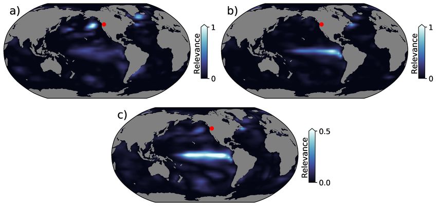
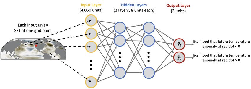
Figure 1: Neural network setup and architecture for predicting the average sign of the temperature
anomalies over Seattle based on sea-surface temperatures (SSTs) 3 months prior.

the chaotic nature of the atmosphere is fully realized, and skillful predictions are very difficult.
However, the societal need for subseasonal and seasonal forecasts is acute: providing any useful
climate information several weeks in advance may have enormous benefits [2].
To break the deadlock on this problem, Earth scientists have come to understand that while skillful
prediction in general is mathematically intractable on subseasonal-to-seasonal timescales, certain
atmospheric processes or configurations of the Earth system can be leveraged to make accurate
subseasonal predictions. While these states are not always present at a given moment in time, when
they are, scientists have the opportunity to use them to make skillful predictions: we call these
instances forecasts of opportunity. As scientists studying this problem, our goal is two-fold: (1)
we must leverage the predictability of forecasts of opportunity to fully extract useful and accurate
predictions, and (2) we must work to identify when forecasts of opportunity exist to begin with.
While the use-case presented here is heavily based on an example from [3], multiple domain-specific
applications led by the co-authors are in preparation.

2     Data
Our network takes as input anomalous monthly sea-surface temperatures (SSTs) across the globe
from the Cobe V2 monthly SST anomaly data set [4], which we linearly regrid to a 4 degree by 4
degree grid spacing. The original 1 degree by 1 degree version of the Cobe V2 SST data used here can
be accessed via NOAA ESRL (https://www.esrl.noaa.gov/psd/data/ gridded/data.cobe2.html). Each
gridded map contains 45 latitudinal grid boxes and 90 longitudinal grid boxes, flattened prior to input
into the network as a vector of length 4050. Points over land are included, but are assigned a value of
zero. As output, we use gridded monthly surface air temperature anomalies from the Berkeley Earth
Surface Temperatures (BEST) [5] data set. This data can be accessed at http://berkeleyearth.org/data/.
For our use-case here, we use only the air temperature time series at the grid point closest to Seattle,
Washington (50o N, 240o E).

3     Methods
3.1   Network architecture and training

We set the network up as a standard binary classification problem. The basic fully-connected, feed-
forward network architecture is shown in Fig. 1. The input into the network is the flattened vector of
SST from one month. The network then contains two hidden layers of 8 nodes each. Each hidden
layer is followed by the Rectified Linear Unit (ReLu) activation function. The final output layer
consists of two nodes representing whether anomalous air temperatures at our chosen location (e.g.
near Seattle) is above and below zero. The output layer includes a soft-max layer to convert the
output into likelihoods that sum to 1. The predicted class is computed as the class with the largest
likelihood, or “confidence”: our work will make use of these likelihood values when quantifying
forecasts of opportunity.
The network is trained using the negative log likelihood loss using gradient descent with the Nesterov
accelerated stochastic gradient descent optimizer and Nesterov momentum parameter of 0.9. The
learning rate starts at 0.01 and is decreased to 0.005 after 50 epochs and trained for an additional 250

                                                   2
Figure 2: (solid curve) Accuracy of the neural network on the testing data as a function of the
network confidence threshold. (dashed curve) Fraction of samples with network confidence above
the threshold, and thus, the fraction of samples used to compute the accuracy.
epochs. Given the large input size and substantial spatial correlation of global SSTs, we include L2
regularization (i.e. ridge regularization) to spread the weights across the inputs and reduce overfitting.
We set the L2 parameter to 10.0 between the input layer and first hidden layer, and set it to 0.01
for all other layers. The training set spans all predictions within the year range of 1950-2005 (672
samples), and the testing set spans all predictions from 2006-2019 (168 samples). Input SSTs and
output air temperatures are standardized by subtracting their respective 1980-2009 mean values at
each grid point and linearly detrending each grid point to account to first order for anthropogenic
climate warming. The range of 1980-2009 is a common climate baseline.
For timescales beyond ∼ two weeks, it is standard to predict weather in an aggregate sense (i.e.
averaged over a given time period) to capture lower frequency temperature fluctuations. Thus, we task
the network with classifying the average temperature anomaly over Seattle 3 months in the future,
which we refer to as a “3 month forecast" henceforth. Recall the label associated with each sample
is binary, predicting if the average temperature anomaly will be positive (assigned a label of 1) or
negative (a label of 0).
3.2 Layer-wise relevance propagation (LRP)
Layer-wise relevance propagation (LRP) is a neural network intepretability method that produces a
heatmap of the most relevant parts of the input for a given prediction. The papers which introduced
LRP describe the full method in detail [6, 7]. [3] illustrates the method from the perspective of a
domain scientist, and [8] demonstrates its use for climate change applications.
In short, LRP takes the network output for a specific class (prior to the softmax layer), termed
“relevance”, and propagates the value backward through the network according to a list of propagation
rules. Upon reaching the input layer, the relevance is split across the input units (in our use-case,
the SST vector), where larger values imply that the particular unit is more relevant for that specific
network prediction. Unlike backward optimization, LRP produces a separate heatmap for each
prediction (i.e. sample), and thus, one can explore the unique decision-making process for each
sample. One main use of LRP within the field of computer science appears to be for debugging a
particular network setup or gaining trust in the network’s output [9]. Yet we believe LRP, applied
to particular questions in other scientific domains, stands to be transformative for advancing and
discovering new science, as suggested by [3, 8, 10]. As one example, here we demonstrate how LRP
can provide scientific insight into the physical mechanisms that lead to enhanced predictability of
surface air temperature on subseasonal-to-seasonal timescales.
4 Results
Predictions of the testing samples show an accuracy of 62% (training accuracy of 65%). As discussed
above, we expect some climate states to lead to more predictable behaviour than others, and we
can use the ANN to identify these states via its predicted confidence/likelihood. Fig. 2 shows the
accuracy across the testing samples as a function of the confidence threshold used: as the network
confidence increases, so does the accuracy. For example, the top 50% most confident predictions have
3Figure 3: (a)-(b) Heatmaps of SST from LRP for two example accurate predictions. (c) Average of
LRP heatmaps for accurate predictions in the top 10% most confident predictions across training and
testing samples (N=63).
an accuracy of 63% while the top 10% most confident predictions have an accuracy of 82%. For the
more confident samples performance is much improved compared to 62% accuracy across all testing
samples. That is, the ANN’s predicted confidence acts as a metric for identifying climate states that
are generally more predictable. This sets the stage for our ability to then identify the physical drivers
and mechanisms of these forecasts of opportunity. Of course, the number of samples decreases as
the confidence threshold is increased, suggesting that as we increase our confidence threshold, the
number of opportunities for making a forecast decreases.
While identifying forecasts of opportunity for temperature predictions 3 months into the future is
useful in its own right, scientifically from our perspective it is more interesting to explore the SST
patterns that correspond to these predictions. To do so, we use LRP to generate heatmaps of the most
relevant regions of SST for the ANN’s prediction. Fig. 3a,b show relevance heatmaps for two samples
that produced accurate predictions. The lightest colors show the regions most relevant for the ANN’s
accurate prediction. We observe high relevance in a small region of the midlatitude eastern Pacific
in (a) and over the tropical eastern Pacific in (b) (indicative of the El Nino Southern Oscillation, or
ENSO, a well known driver of midlatitude temperature variability). Note too that, because each LRP
heatmap is computed for each input sample separately, differences between Fig. 3a,b demonstrate the
network refocusing its attention depending on the specific sample.
While Fig. 3a,b show individual samples, Fig. 3c displays the average over many the LRP heatmaps:
here we average over the top 10% most confident predictions that were accurate in training and testing.
That is, we take the mean of those predictions that we might categorized as confident forecasts of
opportunity. The average LRP map shows that the ENSO region emerges as a dominant driver of
predictability, however, individual heatmaps (such as Fig. 3a) indicate that the network uses other
sources as well. Furthermore, these high-relevance regions align well with areas identified in recent
work on the physical mechanisms for temperature prediction on these timescales [3, 11].
5 Concluding Thoughts
We demonstrated how interpretable neural networks can be used to filter through the noise of a chaotic
climate system and identify periods of enhanced predictability, or “forecasts of opportunity”. Physical
insight into the mechanisms behind this enhanced predictability was then gained (e.g. the ENSO
region) by using layerwise relevance propagation to identify the regions of the input (maps of sea-
surface temperatures) that were most relevant for the network’s accurate prediction. We note that this
methodology alone does not account for causation, as the layerwise relevance propagation heatmaps
merely provide the regions in the input that provide predictability. With that said, these heatmaps can
then be interpreted by a domain scientist to further investigate the dynamical mechanisms that may
tie the input to the prediction of the output in a causal sense. This could include investigating the
time evolution of the sample fields that are identified as successful forecasts of opportunity.
4Next steps for this work include exploring additional cost functions and network setups to further
encourage the network to focus on climate states that lead to enhanced predictability, rather than
minimizing the cost function over all samples. Further, future work will focus on continuing to
understand the physical mechanisms in the ocean and atmosphere of the sources of predictability
identified in this study, in Seattle but also at other points around the globe. While we demonstrate
our approach for the atmospheric science domain, this methodology is applicable to a large range of
geoscientific problems.
Broader Impact
The broader impacts of this work within atmospheric science include improving weather and climate
predictions across seasonal to decadal time scales, while more broadly in the geosciences the “forecast
of opportunity” framework is applicable across a wide range applications. Ultimately, accurate and
timely forecasts can save lives and property, while poor forecasts put both in jeopardy. Investors,
farmers, and energy managers all stand to benefit from skillful and useful subseasonal forecasts,
while inaccurate or over-confident forecasts could lead to poor allocation of resources, financial loss,
and food shortages. Thus, extensive testing of any forecast product based on this work is necessary
and essential prior to it being used for any policy and decision-making. Additionally, as the climate
changes with anthropogenic warming and we enter new and less well-understood climate regimes,
models should be constantly reexamined and re-calibrated to the extent possible to ensure they stay
relevant and accurate.
Acknowledgments and Disclosure of Funding
This work is supported by funding from the National Science Foundation under grants AGS-1749261,
2019758, 006784, 2020305, the Department of Energy under grant DE-FG02-97ER25308, and
Fulbright New Zealand.
References
[1] E. N. Lorenz, “Deterministic Nonperiodic Flow,” Journal of the Atmospheric Sciences, vol. 20,
pp. 130–141, Mar. 1963.
[2] National Academies of Sciences and Medicine, Next Generation Earth System Prediction:
Strategies for Subseasonal to Seasonal Forecasts. Washington, DC: The National Academies
Press, 2016.
[3] B. A. Toms, E. A. Barnes, and I. Ebert-Uphoff, “Physically Interpretable Neural Networks for
the Geosciences: Applications to Earth System Variability,” Journal of Advances in Modeling
Earth Systems, June 2020.
[4] S. Hirahara, M. Ishii, and Y. Fukuda, “Centennial-Scale Sea Surface Temperature Analysis and
Its Uncertainty,” Journal of climate, vol. 27, pp. 57–75, Jan. 2014.
[5] R. Rohde, R. A. Muller, R. Jacobsen, E. Muller, S. Perlmutter, A. Rosenfeld, J. Wurtele,
D. Groom, and C. Wickham, “A New Estimate of the Average Earth Surface Land Temperature
Spanning 1753 to 2011,” Geoinformatics & Geostatistics: An Overview, vol. 2013, 2013.
[6] S. Bach, A. Binder, G. Montavon, F. Klauschen, K.-R. Müller, and W. Samek, “On Pixel-Wise
Explanations for Non-Linear Classifier Decisions by Layer-Wise Relevance Propagation,” PloS
one, vol. 10, p. e0130140, July 2015.
[7] G. Montavon, S. Lapuschkin, A. Binder, W. Samek, and K.-R. Müller, “Explaining nonlinear
classification decisions with deep Taylor decomposition,” Pattern recognition, vol. 65, pp. 211–
222, May 2017.
[8] E. A. Barnes, B. Toms, J. W. Hurrell, I. Ebert-Uphoff, C. Anderson, and D. Anderson, “Indicator
patterns of forced change learned by an artificial neural network,” Journal of Advances in
Modeling Earth Systems, vol. n/a, p. e2020MS002195, Aug. 2020.
[9] S. Lapuschkin, S. Wäldchen, A. Binder, G. Montavon, W. Samek, and K.-R. Müller, “Unmask-
ing Clever Hans predictors and assessing what machines really learn,” Nature communications,
vol. 10, p. 1096, Mar. 2019.
5[10] M. Böhle, F. Eitel, M. Weygandt, and K. Ritter, “Layer-Wise Relevance Propagation for
Explaining Deep Neural Network Decisions in MRI-Based Alzheimer’s Disease Classification,”
Frontiers in aging neuroscience, vol. 11, p. 194, July 2019.
[11] A. Capotondi, P. D. Sardeshmukh, E. Di Lorenzo, A. C. Subramanian, and A. J. Miller,
“Predictability of US West Coast Ocean Temperatures is not solely due to ENSO,” Scientific
reports, vol. 9, p. 10993, July 2019.
6You can also read