Image Processing for Digital Photography - Lecture 15: Interactive Computer Graphics Stanford CS248, Winter 2021
←
→
Page content transcription
If your browser does not render page correctly, please read the page content below
Lecture 15:

Image Processing for
Digital Photography
   Interactive Computer Graphics
    Stanford CS248, Winter 2021
A review of image processing
       via convolution

                               Stanford CS248, Winter 2021
Discrete 2D convolution
1
X
(f ⇤ g)(x, y) = f (i, j)I(x i, y j)
i,j= 1
output image filter input image
1
X
= Consider f (i, j)I(x
that is nonzero
i, y onlyj)when: 1 i, j 1
i,j=
Then: 1
1
X
(f ⇤ I)(x, y) = f (i, j)I(x i, y j)
i,j= 1
And we can represent f(i,j) as a 3x3 matrix of values where:
f (i, j) = Fi,j (often called: “filter weights”, “filter kernel”)
Stanford CS248, Winter 2021
Gaussian blur
▪ Obtain filter coefficients by sampling 2D Gaussian function
                               1        i 2 +j 2
            f (i, j) =            2
                                    e     2  2
                            2⇡
▪ Produces weighted sum of neighboring pixels (contribution
   falls off with distance)
   - In practice: truncate filter beyond certain distance for efficiency
  2                         3
   .075 .124 .075
  4.124 .204 .1245
   .075 .124 .075

                                                                   Stanford CS248, Winter 2021
7x7 gaussian blur
Original

Blurred

                    Stanford CS248, Winter 2021
What does convolution with this filter do?
2 3
0 1 0
4 1 5 1 5
0 1 0
Sharpens image!
Stanford CS248, Winter 20213x3 sharpen filter
Original
Sharpened
Stanford CS248, Winter 2021Recall: blurring is removing high frequency
content
Spatial domain result Spectrum
Stanford CS248, Winter 2021Recall: blurring is removing high frequency
content
Spatial domain result Spectrum (after low-pass filter)
All frequencies above cutoff have 0 magnitude
Stanford CS248, Winter 2021Sharpening is adding high frequencies
▪ Let I be the original image
▪ High frequencies in image I = I - blur(I)
▪ Sharpened image = I + (I-blur(I))
“Add high frequency content”
Stanford CS248, Winter 2021Original image (I)
Image credit: Kayvon’s parents
Stanford CS248, Winter 2021Blur(I)
Stanford CS248, Winter 2021I - blur(I)
Stanford CS248, Winter 2021I + (I - blur(I))
Stanford CS248, Winter 2021What does convolution with these filters do?
2 3 2 3
1 0 1 1 2 1
4 2 0 25 40 0 0 5
1 0 1 1 2 1
Extracts horizontal Extracts vertical
gradients gradients
Stanford CS248, Winter 2021Gradient detection filters
Horizontal gradients
Vertical gradients
Note: you can think of a filter as a
“detector” of a pattern, and the
magnitude of a pixel in the output
image as the “response” of the filter
to the region surrounding each pixel
in the input image (this is a common
interpretation in computer vision)
Stanford CS248, Winter 2021Sobel edge detection
▪ Compute gradient response images
2 3
1 0 1
Gx = 4 2 0 25 ⇤ I 2 3
1 0 1
1 0 1 Gx = 4 2 0 25 ⇤ I
2 3 1 0 1
1 2 1
Gy = 4 0 0 0 5⇤I 2 3
1 2 1 1 2 1
Gy = 4 0 0 0 5⇤I
1 2 1
▪ Find pixels with large gradients
q q
2 2 2 2
G= Gx + Gy G= Gx + Gy
Pixel-wise operation on images
Stanford CS248, Winter 2021Cost of convolution with N x N filter?
float input[(WIDTH+2) * (HEIGHT+2)]; In this 3x3 box blur example:
float output[WIDTH * HEIGHT];
Total work per image = 9 x WIDTH x HEIGHT
float weights[] = {1./9, 1./9, 1./9, For N x N filter: N2 x WIDTH x HEIGHT
1./9, 1./9, 1./9,
1./9, 1./9, 1./9};
for (int j=0; jSeparable filter
▪ A filter is separable if can be written as the outer product of
two other filters. Example: a 2D box blur
2 3 2 3
1 1 1 1 ⇥ ⇤
14 1 1
1 1 15 = 4 15 ⇤ 1 1 1
9 3 3
1 1 1 1
- Exercise: write 2D gaussian and vertical/horizontal
gradient detection filters as product of 1D filters (they are
separable!)
▪ Key property: 2D convolution with separable filter can be
written as two 1D convolutions!
Stanford CS248, Winter 2021Implementation of 2D box blur via two 1D convolutions
int WIDTH = 1024
int HEIGHT = 1024;
float input[(WIDTH+2) * (HEIGHT+2)]; Total work per image for NxN filter:
float tmp_buf[WIDTH * (HEIGHT+2)];
float output[WIDTH * HEIGHT];
2N x WIDTH x HEIGHT
float weights[] = {1./3, 1./3, 1./3};
for (int j=0; jBilateral filter
Original After bilateral filter
Example use of bilateral filter: removing noise while preserving image edges
https://www.thebest3d.com/howler/11/new-in-version-11-bilateral-noise-filter.html Stanford CS248, Winter 2021Bilateral filter
Original After bilateral filter
Example use of bilateral filter: removing noise while preserving image edges
http://opencvpython.blogspot.com/2012/06/smoothing-techniques-in-opencv.html Stanford CS248, Winter 2021Bilateral filter Gaussian blur kernel Input image
1 X
BF[I](p) = f (|I(x i, y j) I(x, y)|)G (i, j)I(x i, y j)
Wp i,j
Normalization
(weights should sum to 1)
Re-weight based on difference
For all pixels in support region
in input image pixel values
of Gaussian kernel
1 X
= f (|I(x i, y j) I(x, y)|)G (i, j)
Wp i,j
▪ The bilateral filter is an “edge preserving” filter: down-weight contribution of pixels
on the “other side” of strong edges. f (x) defines what “strong edge means”
▪ Spatial distance weight term f (x) could itself be a gaussian
-
Or very simple: f (x) = 0 if x > threshold, 1 otherwise
Value of output pixel (x,y) is the weighted sum of all pixels in the support region of a
truncated gaussian kernel
But weight is combination of spatial distance and input image pixel intensity difference.
(the filter’s weights depend on input image content)
Stanford CS248, Winter 2021Bilateral filter Pixels with significantly different intensity
as p contribute little to filtered result (they
Input pixel p
are “on the “other side of the edge”
Input image G(): gaussian about input pixel p f(): Influence of support region
G x f: filter weights for pixel p Filtered output image
Figure credit: Durand and Dorsey, “Fast Bilateral Filtering for the Display of High-Dynamic-Range Images”, SIGGRAPH 2002 Stanford CS248, Winter 2021Bilateral filter: kernel depends on image content Figure credit: SIGGRAPH 2008 Course: “A Gentle Introduction to Bilateral Filtering and its Applications” Paris et al. Stanford CS248, Winter 2021
Spatially local vs. frequency local edits
▪ We’ve talked about how to manipulate images in terms of
   adjusting pixel values (localize edits in space to certain pixels)

▪ We’ve talked about how to manipulate images in terms of
   adjusting coefficients of frequencies (localize edits to certain
   frequencies)
   - Eliminate high frequencies (blur)
   - Increase high frequencies (sharpen)

                                                              Stanford CS248, Winter 2021
But what if we wish to localize image edits
both in space and in frequency?
(Adjust certain frequency content of image,
in a particular region of the image)
Stanford CS248, Winter 2021Josephine the Graphics Cat
Stanford CS248, Winter 2021Gaussian pyramid
G2 = down(G1)
G1 = down(G0)
G0 = original image
Each image in pyramid contains increasingly low-pass filtered signal
down() = Gaussian blur, then downsample by factor of 2 in both X and Y dimensions
Stanford CS248, Winter 2021Downsample
▪ Step 1: Remove high frequencies
▪ Step 2: Sparsely sample pixels (in this example: every other pixel)
float input[(WIDTH+2) * (HEIGHT+2)];
float output[WIDTH/2 * HEIGHT/2];
float weights[] = {1/64, 3/64, 3/64, 1/64, // 4x4 blur (approx Gaussian)
3/64, 9/64, 9/64, 3/64,
3/64, 9/64, 9/64, 3/64,
1/64, 3/64, 3/64, 1/64};
for (int j=0; jGaussian pyramid
G0 (original image)
Stanford CS248, Winter 2021Gaussian pyramid
G1
(upsampled back to full res for visualization) Stanford CS248, Winter 2021Gaussian pyramid
G2
(upsampled back to full res for visualization) Stanford CS248, Winter 2021Gaussian pyramid
G3
(upsampled back to full res for visualization) Stanford CS248, Winter 2021Gaussian pyramid
G4
(upsampled back to full res for visualization) Stanford CS248, Winter 2021Gaussian pyramid
G5
(upsampled back to full res for visualization) Stanford CS248, Winter 2021Laplacian pyramid
G1 = down(G0)
G0
Each (increasingly numbered) level in
Laplacian pyramid represents a band
of (increasingly lower) frequency
information in the image
L0 = G0 - up(G1)
[Burt and Adelson 83] Stanford CS248, Winter 2021Laplacian pyramid
L5 = G5
L4 = G4 - up(G5)
L3 = G3 - up(G4)
L2 = G2 - up(G3)
L1 = G1 - up(G2)
Question: how do you
reconstruct original image
from its Laplacian pyramid?
L0 = G0 - up(G1) Stanford CS248, Winter 2021Laplacian pyramid
L0 = G0 - up(G1)
(upsampled back to full res for visualization) Stanford CS248, Winter 2021Laplacian pyramid
L1 = G1 - up(G2)
(upsampled back to full res for visualization) Stanford CS248, Winter 2021Laplacian pyramid
L2 = G2 - up(G3)
(upsampled back to full res for visualization) Stanford CS248, Winter 2021Laplacian pyramid
L3 = G3 - up(G4)
(upsampled back to full res for visualization) Stanford CS248, Winter 2021Laplacian pyramid
L4 = G4 - up(G5)
(upsampled back to full res for visualization) Stanford CS248, Winter 2021Laplacian pyramid
L5 = G5
Stanford CS248, Winter 2021Summary
▪ Gaussian and Laplacian pyramids are image representations
where each pixel maintains information about frequency
content in a region of the image
▪ Gi(x,y) — frequencies up to limit given by i
▪ Li(x,y) — frequencies added to Gi+1 to get Gi
▪ Notice: to boost the band of frequencies in image around
pixel (x,y), increase coefficient Li(x,y) in Laplacian pyramid
Stanford CS248, Winter 2021A digital camera processing pipeline
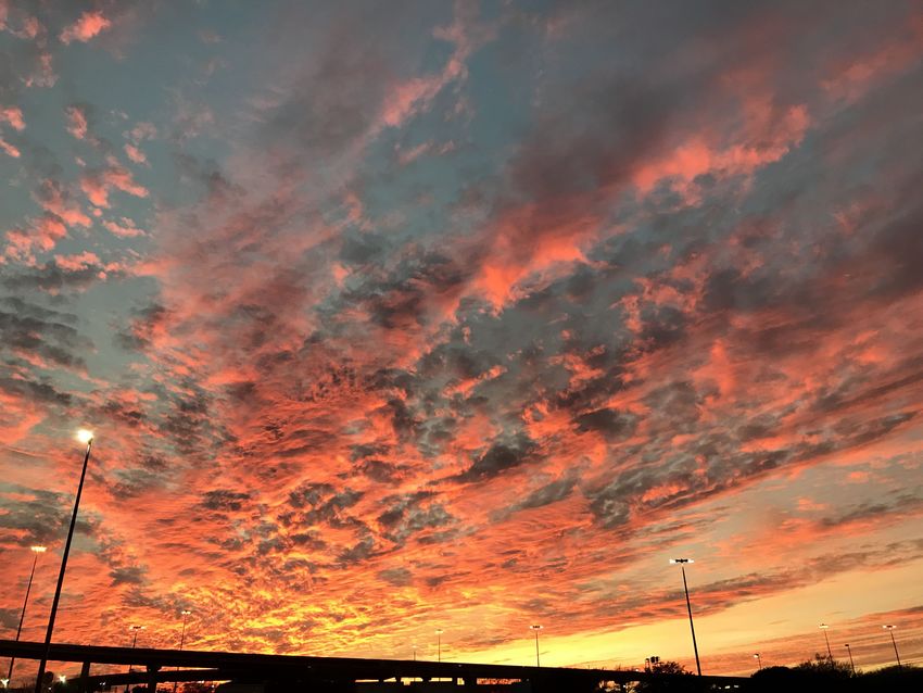
Stanford CS248, Winter 2021Main theme…
The pixels you see on screen are quite different than the values
recorded by the sensor in a modern digital camera.
Image processing computations are now a fundamental aspect
of producing high-quality pictures from commodity cameras.
Sensor output
(“RAW”)
Computation
Beautiful image that
impresses your friends
on Instagram
Stanford CS248, Winter 2021Recall: pinhole camera (no lens)
Scene object 1 Scene object 2
(every pixel measures light
intensity along ray of light
passing through pinhole and
arriving at pixel)
Pinhole
Sensor plane: (X,Y)
Pixel P1 Pixel P2
Stanford CS248, Winter 2021Camera with a lens
Stanford CS248, Winter 2021Camera with a large (zoom) lens
Stanford CS248, Winter 2021Review: out of focus camera Scene focal plane
Scene object 1 Scene object 2
Out of focus camera: rays of
light from one point in scene
do not converge at point on
sensor
Lens aperture
Sensor plane: (X,Y)
Pixel P1 Pixel P2
Previous sensor
plane location
Circle of confusion
Stanford CS248, Winter 2021Bokeh
Stanford CS248, Winter 2021Out of focus camera
Scene focal plane
Scene object 2
Out of focus camera: rays of
light from one point in scene
do not converge at point on
sensor
=
Rays of light from different Lens aperture
scene points converge at
single point on sensor
Sensor plane: (X,Y)
Pixel P1
Previous sensor
plane location
Stanford CS248, Winter 2021Sharp foreground / blurry background
Stanford CS248, Winter 2021Cell phone camera lens(es)
(small aperture)
Stanford CS248, Winter 2021“Portrait mode” (fake depth of field)
▪ Smart phone cameras have small apertures
- Good: thin. lightweight lenses
- Bad:
Synthetic Depth-of-Field
cannot physicallywith
create aaesthetically
Single-Camera Mobile Phone
pleasing photographs with nice
bokeh, blurred background
NEAL WADHWA, RAHUL GARG, DAVID E. JACOBS, BRYAN E. FELDMAN, NORI KANAZAWA, ROBERT
▪ Answer:
CARROLL, simulate behavior of large
YAIR MOVSHOVITZ-ATTIAS, apertureT.lens
JONATHAN using image
BARRON, YAEL processing
PRITCH, and MARC LEVOY,
(hallucinate image formed by large aperture lens)
Google Research
Segmentation
(b) Person segmentation mask
(a) Input image with detected face (c) Mask + disparity from DP (d) Our output synthetic shallow depth-of-field image
Input image /w detected face Scene Depth Generated image
Fig. 1. We present a system that uses a person segmentation mask (b)Estimate
and a noisy depth map computed using (note blurred dual-pixel
the camera’s background. (DP) auto-focus
Blur increases
hardware (c) to produce a synthetic shallow depth-of-field image (d) with a depth-dependent blur on a mobile phone. with
Our system depth) as “Portrait
is marketed
Image
Mode” credit:Google-branded
on several [Wadha 2018] phones.
Stanford CS248, Winter 2021What part of image should be in focus?
Heuristics:
Focus on closest scene region
Put center of image in focus
Detect faces and focus on closest/largest face
Image credit: DPReview:
https://www.dpreview.com/articles/9174241280/configuring-your-5d-mark-iii-af-for-fast-action
Stanford CS248, Winter 2021The Sensor
Stanford CS248, Winter 2021Front-side-illuminated (FSI) CMOS
Pixel pitch:
A few microns
Photodiodes
~50% Fill Factor
Courtesy R. Motta, Pixim Stanford CS248, Winter 2021Metal 4 Courtesy R. Motta, Pixim Stanford CS248, Winter 2021
Color filter array

Courtesy R. Motta, Pixim           Stanford CS248, Winter 2021
Digital image sensor: color filter array (Bayer mosaic)
     ▪ Color filter array placed over sensor
     ▪ Result: different pixels have different spectral response (each pixel
           measures red, green, or blue light)
     ▪ 50% of pixels are green pixels                                    Pixel response curve: Canon 40D/50D

                          Traditional Bayer mosaic
              (other filter patterns exist: e.g., Sony’s RGBE)
                                                                                       f( )
Image credit:
Wikipedia, Christian Buil (http://www.astrosurf.com/~buil/cameras.htm)                              Stanford CS248, Winter 2021
Demosiac
▪ Produce RGB image from mosaiced input image
▪ Basic algorithm: bilinear interpolation of mosaiced values (need 4 neighbors)
▪ More advanced algorithms:
- Bicubic interpolation (wider filter support region… may overblur)
- Good implementations attempt to find and preserve edges in photo
Image credit: Mark Levoy
Stanford CS248, Winter 2021High dynamic range / exposure / noise
Stanford CS248, Winter 2021Denoising
Original
Denoised
Stanford CS248, Winter 2021Denoising via downsampling
Downsample via Downsample via averaging
point sampling (bilinear resampling)
(noise remains) Noise reduced
Stanford CS248, Winter 2021Median filter uint8 input[(WIDTH+2) * (HEIGHT+2)]; uint8 output[WIDTH * HEIGHT]; for (int j=0; j
Saturated pixels   Pixels have saturated (no detail in image)

                                                     Stanford CS248, Winter 2021
Global tone mapping
▪ Measured image values: 10-12 bits/pixel, but common image formats (8-bits/pixel)
▪ How to convert 12 bit number to 8 bit number?
255 255
out(x,y) = f(in(x,y)) low resolution Allow many pixels to “blow
throughout entire out” (detail in dark regions)
range
0 0
212 212
255 255 255
Allow many pixels to
clamp to black (detail
in bright regions)
clamp darkest darks and
brightest brights to reserve
resolution in midtowns
0 0 0
212 212 212
Stanford CS248, Winter 2021Global tone mapping
255
roceedings, August 1997 Allow many pixels to “blow
out” (detail in dark regions)
0
212
255
Allow many pixels to
clamp to black (detail
in bright regions)
Figure 6: Sixteen photographs
0 of a church taken at 1-stop increments from 30
212 borders seen in some of t
glass window, making it especially bright. The blue
Red Stanford CS248, Winter 2021Local tone mapping
IGGRAPH’97 Conference Proceedings, August 1997
▪ Different regions of the image undergo different tone mapping
curves (preserve detail in both dark and bright regions)
(a) (b)
From the SIGGRAPH’97 Conference Proceedings, August 1997
en at 1-stop increments from 30 sec to (d) sec. The sun is directly behind the(e)rightmost stained
Stanford CS248, Winter 2021Local tone adjustment
Short Exposure Medium Exposure Long Exposure
Pixel values
Weight
Masks
(a) Input images with corresponding weight maps
Improve picture’s aesthetics by locally
Figure 2. Exposure
adjusting contrast, boosting darkfusion is guided by weight maps for each inp
a pixel should appear in the final image. These weights reflect de
regions, decreasing bright regions
contrast and saturation. Image courtesy of Jacques Joffre.
(no physical basis at all!)
Combined image
physically-based,(unique
we do notperneed
weights pixel) to worry about calibra- compress the
[Image credit:images
(a) Input tion
Mertens 2007]
with of the camera
corresponding response curve, and keeping(b)track
weight maps of
Fused result which
Stanford CS248,decomp
Winter 2021Challenge of merging images
Four different exposures (corresponding weight masks not shown)
Merged result Merged result
(based on weight masks) (after blurring weight mask)
Notice “banding” since absolute intensity of Notice “halos” near edges
different exposures is different
Stanford CS248, Winter 2021Use of Laplacian pyramid in tone mapping
▪ Compute weights for all Laplacian pyramid levels
▪ Merge pyramids (merge image features), not image pixels
▪ Then “flatten” merged pyramid to get final image
Stanford CS248, Winter 2021Challenges of merging images
Four exposures (weights not shown)
Merged result Merged result
(after blurring weight mask) (based on multi-resolution pyramid merge)
Notice “halos” near edges
Why does merging Laplacian pyramids work better than merging image pixels?
Stanford CS248, Winter 2021Summary
▪ Image processing is now a fundamental part of producing a pleasing photograph
▪ Used to compensate for physical constraints
-
Today: demosaic, tone mapping
-
Other examples not discussed today: denoise, lens distortion correction, etc.
▪ Used to determine how to configure camera (e.g., autofocus)
▪ Used to make non-physically plausible images that have aesthetic merit
Sensor output
(“RAW”)
Computation
Beautiful image that
impresses your friends
on Instagram
Stanford CS248, Winter 2021You can also read