Image Processing, Machine Learning and Visualization for Tissue Analysis
←
→
Page content transcription
If your browser does not render page correctly, please read the page content below
Digital Comprehensive Summaries of Uppsala Dissertations
                from the Faculty of Science and Technology 2025

                Image Processing, Machine
                Learning and Visualization for
                Tissue Analysis

                LESLIE SOLORZANO

    ACTA
UNIVERSITATIS
 UPSALIENSIS    ISSN 1651-6214
                ISBN 978-91-513-1173-9
  UPPSALA       urn:nbn:se:uu:diva-438775
    2021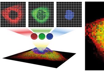
Dissertation presented at Uppsala University to be publicly examined in Room IX,
Universitetshuset, Biskopsgatan 3, Uppsala, Wednesday, 12 May 2021 at 13:00 for the degree
of Doctor of Philosophy. The examination will be conducted in English. Faculty examiner:
Alexandru Cristian Telea (Universiteit Utrecht).

Abstract
Solorzano, L. 2021. Image Processing, Machine Learning and Visualization for Tissue
Analysis. Digital Comprehensive Summaries of Uppsala Dissertations from the Faculty
of Science and Technology 2025. 66 pp. Uppsala: Acta Universitatis Upsaliensis.
ISBN 978-91-513-1173-9.

Knowledge discovery for understanding mechanisms of disease requires the integration of
multiple sources of data collected at various magnifications and by different imaging techniques.
Using spatial information, we can build maps of tissue and cells in which it is possible to
extract, e.g., measurements of cell morphology, protein expression, and gene expression. These
measurements reveal knowledge about cells such as their identity, origin, density, structural
organization, activity, and interactions with other cells and cell communities. Knowledge that
can be correlated with survival and drug effectiveness. This thesis presents multidisciplinary
projects that include a variety of methods for image and data analysis applied to images coming
from fluorescence- and brightfield microscopy.
   In brightfield images, the number of proteins that can be observed in the same tissue section
is limited. To overcome this, we identified protein expression coming from consecutive tissue
sections and fused images using registration to quantify protein co-expression. Here, the main
challenge was to build a framework handling very large images with a combination of rigid and
non-rigid image registration.
   Using multiplex fluorescence microscopy techniques, many different molecular markers
can be used in parallel, and here we approached the challenge to decipher cell classes based
on marker combinations. We used ensembles of machine learning models to perform cell
classification, both increasing performance over a single model and to get a measure of
confidence of the predictions. We also used resulting cell classes and locations as input to a
graph neural network to learn cell neighborhoods that may be correlated with disease.
   Finally, the work leading to this thesis included the creation of an interactive visualization
tool, TissUUmaps. Whole slide tissue images are often enormous and can be associated with
large numbers of data points, creating challenges which call for advanced methods in processing
and visualization. We built TissUUmaps so that it could visualize millions of data points from
in situ sequencing experiments and enable contextual study of gene expression directly in the
tissue at cellular and sub-cellular resolution. We also used TissUUmaps for interactive image
registration, overlay of regions of interest, and visualization of tissue and corresponding cancer
grades produced by deep learning methods.
   The aforementioned methods and tools together provide the framework for analysing and
visualizing vast and complex spatial tissue structures. These developments in understanding
the spatial information of tissue in different diseases pave the way for new discoveries and
improving the treatment for patients.

Keywords: Image processing, data analysis, machine learning, visualization, microscopy

Leslie Solorzano, Department of Information Technology, Division of Visual Information and
Interaction, Box 337, Uppsala University, SE-751 05 Uppsala, Sweden.

© Leslie Solorzano 2021

ISSN 1651-6214
ISBN 978-91-513-1173-9
urn:nbn:se:uu:diva-438775 (http://urn.kb.se/resolve?urn=urn:nbn:se:uu:diva-438775)
Dedicated to all women whose efforts led to our freedoms and rights
                         and to all the women who will come after.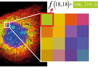
List of papers

This thesis is based on the following papers, which are referred to in the text
by their Roman numerals.

   I   Solorzano, L., Partel, G., Wählby, C. “TissUUmaps: Interactive
       visualization of large-scale spatial gene expression and tissue
       morphology data”, Bioinformatics OUP, August 1, 2020.

  II   Solorzano, L., Pereira, C., Martins, D., Almeida, R., Carneiro, F.,
       Almeida, G., Oliveira, C., Wählby, C. “Towards automatic protein
       co-expression quantification in immunohistochemical TMA slides”,
       IEEE Journal of Biomedical and Health Informatics, July 13, 2020.

 III   Solorzano, L. Almeida, G., Mesquita, B., Martins, D., Oliveira, C.,
       Wählby, C. “Whole slide image registration for the study of tumor
       heterogeneity”, Computational Pathology and Ophthalmic Medical
       Image Analysis. COMPAY 2018, published in Lecture Notes in
       Computer Science book series (LNCS, volume 11039), September 14,
       2018.

 IV    Solorzano, L. Wik, L., Bontell. T.O., Klemm. A. H. , Wang, Y.,
       Öfverstedt, J., Jakola, A.S., Östman A., Wählby, C. “Machine learning
       for cell classification and neighborhood analysis in glioma tissue”,
       under review, February, 2021.

Reprints of papers I,II and IV were made without the need for permission
since they are published under an open-access licence. Reprint of paper III
was made with permission from the publishers.
   For paper I, Solorzano, L. is the main contributor to the software
development and architecture. Solorzano wrote the paper with inputs from
the co-authors.
   For paper II, Solorzano, L. is the main contributor to the image analysis
methods and software development. Solorzano wrote the paper with inputs
from the co-authors.
   For paper III, Solorzano, L. is the main contributor to the image analysis
methods and software development. Solorzano wrote the paper with inputs
from the co-authors.
   For paper IV, Solorzano, L. is the main contributor to the image analysis
methods, machine learning experiment design, software development and
visualization. Solorzano wrote the paper with inputs from the co-authors.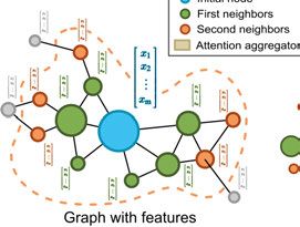
Related work

In addition to the papers included in this thesis, the author has also written or
contributed to the following publications:

R1    Partel, G., Hilscher, M. M., Milli, G., Solorzano, L., Klemm, A. H.,
      Nilsson, M., Wählby, C. “Automated identification of the mouse
      brain’s spatial compartments from in situ sequencing data”, BMC
      Biology, October 19, 2020.

R2    Ström, P., Kartasalo, K., Olsson, H., Solorzano, L., Delahunt, B.,
      Berney, D.M., Bostwick, D.G., Evans, A.J., Grignon, D.J., Humphrey,
      P.A., Iczkowski, K.A., Kench, J.G., Kristiansen, G., vanderKwast,
      T.H., Leite, K.R.M., McKenney, J.K., Oxley, J., Pan, C.-Chen ,
      Samaratunga, H., Srigley, J.R., Takahashi, H., Tsuzuki, T., Varma, M.,
      Zhou, M., Lindberg, J., Bergström, C., Ruusuvuori, P., Wählby, C.,
      Grönberg, H., Rantalainen, M., Egevad, L., Eklund, M. “Artificial
      intelligence for diagnosis and grading of prostate cancer in biopsies: a
      population-based, diagnostic study”, The Lancet Oncology, January 8,
      2020.

R3    Gupta, A., Harrison, P., Wieslander, H., Pielawski, N., Kartasalo, K.,
      Partel, G., Solorzano, L., Suveer, A., Klemm, A., Spjuth, O., Sintorn,
      I., Wählby, C., “Deep learning in image cytometry: a review”,
      Cytometry Part A, December 19, 2018.

During the course of this research, the author has also contributed to the
following pre-publications and conferences

 P1   Andersson, A., Partel. G., Solorzano, L., Wählby, C.
      “Transcriptome-Supervised Classification of Tissue Morphology Using
      Deep Learning”, IEEE 17th International Symposium on Biomedical
      Imaging (ISBI), April 2020.

 P2   Bombrun. M., Ranefall. P., Lindblad. J., Allalou. A., Partel. G.,
      Solorzano, L. Qian. X., Nilsson. M., Wählby, C. “Decoding gene
      expression in 2D and 3D”, Scandinavian Conference on Image
      Analysis (SCIA) 2017, published in Lecture Notes in Computer Science
      book series (LNCS, volume 10270), June 12, 2017.
Contents
1 Background . . . . . . . . . . . . . . . . . . . . . . . . . . . . . . . . . . . . . . . . . . . . . . . . . . . . . . . . . . . . . . . . . . . . . . . . . . . . . . . . . . . . . . . . . . . . . . . . 11
1.1 Motivation . . . . . . . . . . . . . . . . . . . . . . . . . . . . . . . . . . . . . . . . . . . . . . . . . . . . . . . . . . . . . . . . . . . . . . . . . . . . . . . . . . . . . . . 11
1.2 Digital image analysis . . . . . . . . . . . . . . . . . . . . . . . . . . . . . . . . . . . . . . . . . . . . . . . . . . . . . . . . . . . . . . . . . . . . 12
1.3 Data analysis . . . . . . . . . . . . . . . . . . . . . . . . . . . . . . . . . . . . . . . . . . . . . . . . . . . . . . . . . . . . . . . . . . . . . . . . . . . . . . . . . . . 12
1.4 Machine learning and deep learning . . . . . . . . . . . . . . . . . . . . . . . . . . . . . . . . . . . . . . . . . . . . . 13
1.5 Quantitative microscopy . . . . . . . . . . . . . . . . . . . . . . . . . . . . . . . . . . . . . . . . . . . . . . . . . . . . . . . . . . . . . . . . 13
1.6 Combining multiple sources of information . . . . . . . . . . . . . . . . . . . . . . . . . . . . . . . . 14
1.7 Visualization . . . . . . . . . . . . . . . . . . . . . . . . . . . . . . . . . . . . . . . . . . . . . . . . . . . . . . . . . . . . . . . . . . . . . . . . . . . . . . . . . . . 14
2 Quantitative microscopy . . . . . . . . . . . . . . . . . . . . . . . . . . . . . . . . . . . . . . . . . . . . . . . . . . . . . . . . . . . . . . . . . . . . . . . . . . 16
2.1 Microscopy techniques . . . . . . . . . . . . . . . . . . . . . . . . . . . . . . . . . . . . . . . . . . . . . . . . . . . . . . . . . . . . . . . . . . 16
2.1.1 Fluorescence microscopy . . . . . . . . . . . . . . . . . . . . . . . . . . . . . . . . . . . . . . . . . . . . . . . . 16
2.1.2 Brightfield microscopy . . . . . . . . . . . . . . . . . . . . . . . . . . . . . . . . . . . . . . . . . . . . . . . . . . . . 18
2.1.3 Multiplexed analysis . . . . . . . . . . . . . . . . . . . . . . . . . . . . . . . . . . . . . . . . . . . . . . . . . . . . . . . . 18
2.2 Challenges of using microscopy data . . . . . . . . . . . . . . . . . . . . . . . . . . . . . . . . . . . . . . . . . . . 19
3 Image analysis . . . . . . . . . . . . . . . . . . . . . . . . . . . . . . . . . . . . . . . . . . . . . . . . . . . . . . . . . . . . . . . . . . . . . . . . . . . . . . . . . . . . . . . . . . . 22
3.1 Digital images . . . . . . . . . . . . . . . . . . . . . . . . . . . . . . . . . . . . . . . . . . . . . . . . . . . . . . . . . . . . . . . . . . . . . . . . . . . . . . . . 22
3.2 Image segmentation . . . . . . . . . . . . . . . . . . . . . . . . . . . . . . . . . . . . . . . . . . . . . . . . . . . . . . . . . . . . . . . . . . . . . . . 22
3.2.1 Object segmentation . . . . . . . . . . . . . . . . . . . . . . . . . . . . . . . . . . . . . . . . . . . . . . . . . . . . . . . . 22
3.2.2 Region segmentation . . . . . . . . . . . . . . . . . . . . . . . . . . . . . . . . . . . . . . . . . . . . . . . . . . . . . . . 24
3.3 Image registration . . . . . . . . . . . . . . . . . . . . . . . . . . . . . . . . . . . . . . . . . . . . . . . . . . . . . . . . . . . . . . . . . . . . . . . . . . . 24
3.4 Color transformation and unmixing . . . . . . . . . . . . . . . . . . . . . . . . . . . . . . . . . . . . . . . . . . . . . . 25
3.5 Open source software tools for image analysis . . . . . . . . . . . . . . . . . . . . . . . . . . . . 26
4 Quantitative Data Analysis . . . . . . . . . . . . . . . . . . . . . . . . . . . . . . . . . . . . . . . . . . . . . . . . . . . . . . . . . . . . . . . . . . . . . . . 28
4.1 Classification . . . . . . . . . . . . . . . . . . . . . . . . . . . . . . . . . . . . . . . . . . . . . . . . . . . . . . . . . . . . . . . . . . . . . . . . . . . . . . . . . . 28
4.2 Unsupervised learning . . . . . . . . . . . . . . . . . . . . . . . . . . . . . . . . . . . . . . . . . . . . . . . . . . . . . . . . . . . . . . . . . . . 29
4.2.1 Clustering . . . . . . . . . . . . . . . . . . . . . . . . . . . . . . . . . . . . . . . . . . . . . . . . . . . . . . . . . . . . . . . . . . . . . . . . . 29
4.2.2 Contrastive learning . . . . . . . . . . . . . . . . . . . . . . . . . . . . . . . . . . . . . . . . . . . . . . . . . . . . . . . . . 31
4.2.3 Curse of dimensionality . . . . . . . . . . . . . . . . . . . . . . . . . . . . . . . . . . . . . . . . . . . . . . . . . . 31
4.3 Dimensionality reduction . . . . . . . . . . . . . . . . . . . . . . . . . . . . . . . . . . . . . . . . . . . . . . . . . . . . . . . . . . . . . . 32
4.4 Machine learning and Deep Learning . . . . . . . . . . . . . . . . . . . . . . . . . . . . . . . . . . . . . . . . . . . 33
4.4.1 History . . . . . . . . . . . . . . . . . . . . . . . . . . . . . . . . . . . . . . . . . . . . . . . . . . . . . . . . . . . . . . . . . . . . . . . . . . . . . . 33
4.4.2 Decision trees . . . . . . . . . . . . . . . . . . . . . . . . . . . . . . . . . . . . . . . . . . . . . . . . . . . . . . . . . . . . . . . . . . . 34
4.4.3 Deep learning . . . . . . . . . . . . . . . . . . . . . . . . . . . . . . . . . . . . . . . . . . . . . . . . . . . . . . . . . . . . . . . . . . . 35
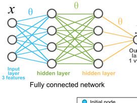
4.4.4 Neural networks . . . . . . . . . . . . . . . . . . . . . . . . . . . . . . . . . . . . . . . . . . . . . . . . . . . . . . . . . . . . . . . 364.4.5 GNNs and node representations ..................................... 36
5 Data visualization . . . . . . . . . . . . . . . . . . . . . . . . . . . . . . . . . . . . . . . . . . . . . . . . . . . . . . . . . . . . . . . . . . . . . . . . . . . . . . . . . . . . . . 39
5.1 Maps of high resolution data . . . . . . . . . . . . . . . . . . . . . . . . . . . . . . . . . . . . . . . . . . . . . . . . . . . . . . . . . 40
5.2 Digital color . . . . . . . . . . . . . . . . . . . . . . . . . . . . . . . . . . . . . . . . . . . . . . . . . . . . . . . . . . . . . . . . . . . . . . . . . . . . . . . . . . . . 42
5.3 From data to visualization . . . . . . . . . . . . . . . . . . . . . . . . . . . . . . . . . . . . . . . . . . . . . . . . . . . . . . . . . . . . . 44
5.4 Open source software libraries . . . . . . . . . . . . . . . . . . . . . . . . . . . . . . . . . . . . . . . . . . . . . . . . . . . . . . 46
6 Contributions / Methods and applications / per paper . . . . . . . . . . . . . . . . . . . . . . . . . . . . . 47
6.1 Paper I - TissUUmaps: Interactive visualization of large-scale
spatial gene expression and tissue morphology data . . . . . . . . . . . . . . . . . . . 48
6.2 Paper II - Towards automatic protein co-expression
quantification in immunohistochemical TMA slides . . . . . . . . . . . . . . . . . . . 49
6.3 Paper III - Whole slide image registration for the study of
tumor heterogeneity . . . . . . . . . . . . . . . . . . . . . . . . . . . . . . . . . . . . . . . . . . . . . . . . . . . . . . . . . . . . . . . . . . . . . . . 49
6.4 Paper IV - Machine learning for cell classification and
neighborhood analysis in glioma tissue . . . . . . . . . . . . . . . . . . . . . . . . . . . . . . . . . . . . . . . . 50
7 Conclusions and future work .................................................................... 51
Summary in Swedish ....................................................................................... 53
Summary in Spanish ........................................................................................ 56
Acknowledgements .......................................................................................... 59
References ........................................................................................................ 611. Background
The most exciting phrase to hear in science, the one that heralds
the most discoveries, is not “Eureka!” but “That’s funny...”
I SAAC A SIMOV
Prolific writer, scientist, professor, humanist
1.1 Motivation
Humans are curious creatures and like to see patterns and understand the way
the world works. Humanity works on mapping the cosmos, mapping planet
earth (and more recently Mars as well), and also on mapping biological tissue
and cells. Once mapped, relationships between these entities can also be
studied and so can their behaviors and their influence in the progression and
function of disease. One of the most important tools for that purpose is
digital image analysis along with data analysis and data visualization.
Understanding how diseases work and how to stop them is key and is today
being used for personalized treatments, for example targeted cancer therapy.
The myriad of techniques for imaging, methods for analysis and
mathematical models has made it possible to study the same phenomenon
from different points of view, it is important to be able to combine the study
from a single method with many others. This is only possible today thanks to
advanced technology and efficient use of computational resources to help
reduce the load and increase the throughput and confidence in the results.
This thesis is the summary of an interdisciplinary work with the goal of
helping researchers in the medical and biological fields to answer questions
in their domains through the analysis of digital images and the data that can
be extracted from them. This can be achieved with computer science which
allows the understanding of mathematical models and their efficient
implementation and also provides the tools for creating software where the
exploration, processing and visualization of data is possible. [1].
In Figure 1.1 I wanted to show a summary of all the steps in an image and
data analysis project applied to biology. I trust I manage to convey how they
all play a part on gaining insight and knowledge. Also how every project and
question requires the integration with other projects and sources of data that
came before and have gone through the same process.
111.2 Digital image analysis Digital images are pictures or photographs captured by electronic sensors. In digital cameras tiny sensors detect and measure light. This measurement is turned into color or intensity that will be associated with one pixel. Digital images are composed of many of such pixels. Digital cameras such as the ones in mobile phones and even more advanced ones, are coupled to microscopes which allow to record the observed micro-scenes, akin to observing stars through telescopes or buildings and roads in satellite imagery, a plethora of objects, be it stars, buildings or cells, are organized and working together to perform different activities with different goals. In all of these images, a demarcation of objects of interest is usually performed and several features or characteristics are computed from them, for example finding which pixels compose different instances of cells, and getting information about size, shape, color, location, individual and relative to others. Tissue is composed of many such cells, and their spatial organization can inform about the location or the status of a disease. Another example is to find gene expression in an image, where small objects within a cell inform of the genetic profile which characterizes a cell and its function. 1.3 Data analysis In order to make sense of the information gathered from many sources about an event or disease, there needs to be a workflow to analyze, classify, organize and represent the knowledge that can be learned from it. Samples can be organized by the types of their cells or even by the types of interactions between their cells. Cells can be classified by their properties, and such properties can come from many sources and in many shapes, 2D points, 3D points, ND points, connected points, disconnected points, grids etc. Data analysis encompasses methods, and efficient algorithms to use statistics and mathematical modelling to extract understand the information extracted from the images. Methods can range from simple (but not less interesting) to intricate, from linear regression to deep neural networks. The goal of data analysis is to be able to categorize or model the different features of tissue, cells and gene expression. Data analysis also includes the models of transformations between all the different data modalities. Microbiologist works in micrometers and nanometers and image analysts work in pixels, data and image analysis include ways to transform from one space into the other. 12
1.4 Machine learning and deep learning
Some of the most commonly used methods today are machine learning (ML)
methods. Contrary to the popular belief, these methods are not new. Already
in 1958 the perceptron was proposed [2] as a model for supervised learning.
But with the advent of more powerful computers these methods have also
developed into enormous and complicated models.
   ML is basically a form of applied statistic which takes advantage of the
recent computational tools to statistically estimate complicated functions. ML
has the challenge of fitting models to the data and the challenge of finding
patterns that generalize to new data. Unlike pure statistic, it started with little
emphasis on proving confidence intervals around the models and functions but
recently a whole field has been trying to combat this, it is called “explainable
AI”, which develops methods to unveil the ML blackbox.
   Most ML algorithms can be divided into two categories: supervised and
unsupervised learning. At the heart of ML is optimization, and the most used
algorithm is called stochastic gradient descent. Borrowing from optimization,
ML combines optimization algorithms, a cost function, a model and a dataset.
Through time, more data, more sources and more complex questions brought
to light the limitations of traditional ML to generalize to new scenarios. These
challenges motivated the development of deep learning (DL) algorithms.
   ML and DL can be used, for example, to detect objects in images, to
characterize those objects or to classify them. These methods can be used in
ND disconnected points, or in graphs or in grids, such as images. It has
become a standard component of data analysis.

1.5 Quantitative microscopy
Digital image analysis has offered unique opportunities in the field of
microscopy. Observations made in microscopes can be recorded and stored
digitally to be observed at any time without the need to store the biological
sample. In these images a number of measurements can be extracted,
allowing the observation of detailed parts of cells, detailed structures in tissue
and even molecular structures, all ranging from micrometers to nanometers.
   Being able to analyze, categorize and extract knowledge from biological
samples gave rise to digital pathology where the nature and mechanisms of
disease can be studied by imaging samples of biopsies and providing insights
at a very fast pace.
   Quantitative microscopy and digital pathology have now advanced at an
amazing speed, incorporating fast and efficient computation strategies, use of
ML and DL and advanced autonomous scanners with hardware to perform
chemical staining procedures and handling optics, lenses and lasers which are
needed to capture the images.

                                                                                13
1.6 Combining multiple sources of information A single event or object can be observed with different kinds of microscopy, in different resolutions and different times. For example, the type of a cell can be determined by knowing the proteins it expresses, the genes that are active in it, its shape, its location and its neighbors. All of that information comes from different sources which work in different dimensions, units, types and fields of view. During the course of this research, tools and methods were developed to combine these different sources of information and explore it in a single convenient point of reference. 1.7 Visualization With the arrival of big data and high throughput experiments, images can be created by the million, and information has to be summarized and the most important aspects have to be brought to light. This is where image analysis, data analysis come in. Images can be selected, processed and summarized to then become candidates for visualization. Results obtained after processing of images and data are key to gain knowledge. Excellent visualization is thoughtful design and presentation of interesting data, it’s a matter of content, statistics and design [3]. It is achieved when complex ideas can be communicated with clarity, precision and efficiency. A visualization of an idea should give the viewer the greatest number of ideas in the shortest time with the least amount of objects and the smallest space. Graphical excellence is nearly always multivariate and graphical excellence requires telling the truth about the data. In more recent times, with the available computational infrastructure, GPUs, and affordable advanced technology, data can (and is almost expected to) be explored interactively, where a user can continuously input parameters and a more localized view of the results can be obtained. Such exploration is useful to gain further knowledge and highlight new ideas of previously unseen relationships in a field, like biology. 14
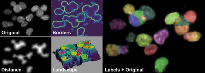
Figure 1.1. Image processing and data analysis. Knowledge can be derived through
methods and models applied to images and data. Objects and regions can be
segmented, quantified and classified. If more data coming from other sources is
available it can be brought together. Such data has usually undergone a similar process
of discovery. The results can be visualized on top of the original image data and
data can be explored, analyzed and modeled thus answering a question, furthering the
knowledge that allows for posing newer more relevant questions. Here an example
is shown. When a question arises, tissue samples can be collected and arranged on
a glass slide and stained. The image depicts small pieces of tissue arranged in a
micro array. Each piece can contain thousands of cells. Cell nuclei are segmented
in fluorescence microscopy images and associated biomarkers are quantified within
the area marked by the nuclei and this quantification serves as a set of features to
classify the nuclei. Once a class is defined it could be related to other data such as
gene expression expected to appear only in specific classes or regions, or perhaps the
nuclei can be observed under a different kind of microscopy. Once all information is
gathered it can be observed, validated and interpreted to answer a biological question
or describe a phenomenon or mechanisms of disease. New insights can inspire new
questions and an even more targeted imaging can be done and the process can begin
again.

                                                                                    15
2. Quantitative microscopy There are two main kinds of microscopy, electron and optical. I will focus on optical which uses illumination and lenses to direct and filter light. Biological samples are usually transparent which means they have to be prepared and stained in order to be visible before going into the microscope or scanner. Different microscopy techniques require very specialized staining and chemistry before they are ready to be imaged. Microscopy images that contain a micrometer thin slice of a full piece of tissue mounted on a glass slide are usually referred to as Whole Slide Images (WSI). Other images contain arrays of smaller circular pieces of tissue resulting from punched out pieces from tissue collected and arranged in a paraffin block, and then sliced, mounted on glass and stained. These images are called Tissue Microarrays (TMA). In this chapter I present the type of microscopy used to capture the images in the datasets for the different projects I was involved in and the numerous challenges presented when working with microscopy images. 2.1 Microscopy techniques 2.1.1 Fluorescence microscopy To capture an image in fluorescence microscopy, a sample has to be stained. Occasionally the imaged sample can contain self-fluorescent materials. Once the stain has attached to its intended target the sample is illuminated and excited fluorescent molecules (fluorophores) will emit light that is captured by the sensors that create the digital image [4]. Using different filters for different wavelengths, each stain can be captured in a different image channel. The most frequently used stain is that of nuclei, generally obtained using 4’6-diamidino-2-phenylindole (DAPI). Images of this stain is used to detect cell nuclei which are later associated with complete cell objects [5]. The area outlined by the nucleus and cell objects is used to extract the rest of the cell features in all the other channels of an image. Amongst fluorescence microscopy there are many subgroups related to the particular molecules to which stains attach to, or the kind of light used to excite them, or the kind of chemical treatment used, or the pathways the light follows to image the sample. Multiplexed immunofluorescence (mIF or mIHC) is a kind of preparation of a sample so that using fluorescence microscopy an image with information on multiple molecular markers can be 16
Figure 2.1. Illustration of the process of image acquisition in fluorescence microscopy.
A sample, cell or tissue is lit with a light source, the reflected or emitted light passes
through band filters to separate into different channels (3 are depicted but there can
be several). Each channel is grayscale but can be pseudo colored for visualization
purposes. When combined using RGB space, the full cell can be observed. Each pixel
x contains the channel intensities f (x)

obtained. A fluorophore is attached to an antibody (hence the immuno-) and
this antibody targets a specific protein of interest. Wherever this protein is
present, the fluorophore attached will light up when excited and the result is
an image where the location of the protein is mapped [6, 7]. Using mIF, up to
eight different proteins can be imaged in the same sample, and the goal is to
observe and characterize cells by the combination of proteins they express.
WSI and TMA contain from thousands to hundreds of thousands of cells. We
work with mIF in paper IV. Recently a technique called co-detection by
indexing (CODEX)[8] allows the simultaneous study of up to fifty
biomarkers at the cost of being low throughput. This means that it is possible
to quantify up to fifty markers for every cell.
   Tissue and cells can be characterized by protein expression but also by
gene expression. Using specialized chemistry and fluorescence microscopy,
single mRNA molecules can be detected, amplified and sequenced directly in
the tissue, preserving the natural histological context, and allowing the
connection of the mRNA sequence with spatial information. This method is
called in situ sequencing [9]. Gene expression images can be usually
accompanied by a DAPI stain channel where it is possible to associate
individual gene expression to a specific nucleus. Specific combinations of
RNA molecules can characterize a cell or indicate about its behavior or
membership to a particular class. Millions of data points arise as a result of in
situ gene expression mapping.
   Hundreds of thousands of cells and millions of gene expression points are
part of the data that is used for quantitative analysis of tissue behavior in
conditions of disease and for survival studies. They are big data and require
special image and data analysis techniques, along with specialized software
to explore and visualize. We use gene expression data in paper I.

                                                                                      17
2.1.2 Brightfield microscopy In this type of microscopy, tissue is illuminated using a white light source, commonly a halogen lamp in the microscope stand. Unstained tissue will appear as transparent (background color). For this reason the tissue has to be sliced into thin sections, fixated and then stained to display the desired object. Thin sections are required so that light can shine through, to have depth of focus and for the stain to reach and bind to its target. The transmitted light will result in a colored image that can be viewed or captured with a digital camera. The specimen is illuminated from below and observed from above. Two of the most common staining techniques are called Haematoxylin Eosine (H&E) and Haematoxylin Diaminobenzidine (HDAB). In H&E, acidic cellular components react with a basic stain, H, while basic components react with an acidic stain E. H&E staining is not specific to a molecule, it is used to reveal the distribution of cells and of elements within cells. On the other hand, in immunohistochemistry (IHC), DAB staining is used to reveal the existence and localization of a target protein in the context of different cell types, biological states, or sub-cellular localization within complex tissues. [10].Brightfield microscopy, H&E and HDAB are the most common techniques by pathologists to observe the morphology of tissue, distribution of cells and structures and characteristics of cells that are indicatives of specific diseases an behaviours [11]. We use IHC HDAB images in papers II and III. 2.1.3 Multiplexed analysis Fluorescence, brightfield and other kinds of microscopy provide different kinds of information that, when combined, reveal new information that might not be possible to obtain with a single technique. H&E and IHC are more commonly used to characterize a disease through the texture and intensities which reveals the overall scaffold and structure of the tissue. Fluorescence can indicate the location and amount of more than one marker of interest at once, thus giving clues on what proteins may interact or be involved in the same cellular (or sub cellular) process. When using fluorescence data overlaid on brightfield data it provides insight on the mechanisms of the activity that is happening in the areas detected by H&E [12], for example, pathologists can detect tumor areas in H&E images and the proteins can be quantified in fluorescence images. More recently overlaid fluorescence data has been used as a label for supervised machine learning methods as opposed to labeling the H&E stained images manually [13]. Additionally new exploratory methods translate H&E staining to mIF or to IHC [14], and from mIF imaging, pseudo IHC or H&E colored images can be created to allow the transfer of knowledge from traditional histopathology to fluorescence imaging [15]. Figure 2.2 illustrates the different kinds of microscopy used in 18
Figure 2.2. Illustration of a piece of tissue under different microscopy modalities and
stainings. A and B are IHC stained with HDAB. A) and B) are two different images
from two different but consecutive tissue slices each targeting a different protein by
IHC, therefore there are two different patterns C) is a synthetic recreation of H&E
staining, the darker purple spots are nuclei. D) is a synthetic recreation of fluorescent
staining, blue corresponds to nuclei, and red and green for the same proteins in A and
B. In the studies of coexpression of multiple markers it is preferable to have mIF but
when there is no access to it, several IHC can be performed on consecutive slices.
E) shows nuclei in white and their accompanying gene expression. The small dotted
colors represent the first base of an mRNA sequence (ACGT). One cell is displayed
with all its bases. This is an example of bringing together different images to extract
information

this thesis. It shows a synthetic recreation of an H&E and mIF view from real
IHC images to depict how the same tissue would look under different
modalities. Additionally in (E) it shows a view of in situ sequencing gene
expression. The nuclei can be observed in white and are physically as big as
the nuclei represented in blue dots in fluorescence (D). The scale bars
indicate that the view of in situ sequencing is of higher magnification than
A,B,C and D.

2.2 Challenges of using microscopy data

Figure 2.3. Process of loading and viewing a TMA. For a particular location and zoom
level a request is made for the tiles that cover the desired view. A server software (local
or remote) receives the request and procures the tile either by creating a new image or
loading an existing one.

                                                                                        19
Despite depicting a relatively small piece of physical biological tissue, microscopy images are obtained at a very high resolution that allows us to observe individual cells to a high level of detail. This results in one of the major challenges of working with microscopy: the size of the image. While the image from a phone can be on average 2000x1500 pixels, images in microscopy can range from 5 to 50 times that, resulting in 25 to 2500 times the amount of pixels, which is why they are referred to as gigapixel images. WSI and TMA images can be a single channel or a multichannel or multispectral image, where several wavelengths can be represented. To address the size problem, images are saved in different levels of detail, different fields of view and different image compression of the same sample in a pyramidal scheme[16], resulting in a file that contains images of different sizes inside in the form of tiles. This solves the problem of structure of data but introduces a new problem: hundreds of different formats created by all microscope vendors. Science is gradually becoming more open [17] and formats are being standardized [18, 19] and more specialized libraries are now able to load big images into memory. Taking advantage of the pyramidal scheme, microscopy images become distributed data, it can be streamed or served, so that it doesn’t have to be stored locally. For that purpose various servers were created to serve microscopy tiles belonging to one of several levels of the pyramid. This also means that specialized processing is required for this data since it has to be done either in downsampled levels in the pyramid or in tiled high resolution patches or in a multilevel fashion. Challenges are several and interconnected and anybody interfacing with a system that produces this kind of data has to, undoubtedly, make design choices when performing any kind of research project involving microscopy. Given the image size a researcher can choose to store images locally or in a specialized repository. Given the microscope, only certain formats and readers (and sometimes writers) are available. For processing needs, the researcher must decide if the pyramid should be accessed in an offline fashion: the pyramid will be stored in separate tiles for quick access at the cost of space (and cost of transfer if served), or online: if the pyramids should be stored compressed to save space at the cost of creating the tiles every time they are needed and served. Images inside the pyramids usually contain known file formats and algorithms like jpg, png, tiff, jpeg2000, all with different parameters. There are also private ones. Most of the time pyramids can be read but not stored if unlicensed meaning that after processing a pyramid has to be created in a different open format. Libraries that have been created to deal with these specific biological pyramidal images in local environments are OpenSlide[20], Bio-formats[21], slideio [22]. Libraries that are able to open pyramids of any kind are VIPS[23] and BigTiff/Libtiff. They are mostly developed in C, C++, Python and Java programming languages. 20
To serve images, whether they are stored locally or stored in the cloud,
software like the IIPImage server was created by the International Image
Interoperability Framework [24]. Web servers like Apache can receive http
requests for tiles.
   Online viewers that can read local and IIIF served images are
OpenSeadragon[25], Zoomify[26], and OpenLayers[27].
   To give an idea of the image sizes that microscopy data uses, the smallest
size displayed so far in TissUUmaps (the visualization software developed
during the course of this thesis) is of 9000 times 6000 pixels. The biggest is
110000 times 100000 pixels. In comparison, most mobile phones and hand
held devices used by the general public today reach 4000 times 3000 pixels.

                                                                           21
3. Image analysis In digital images as the ones coming from microscopes, objects of interest can be detected as specific ranges in the signal. Signals can be unmixed into components. Patterns can be found in them, which represent distinctive tissue characteristics. This approach can be used to obtain meaningful information in fields like microscopy. To achieve this goal, in this thesis, workflows have been developed for object detection, object classification and image description. This chapter will present a recapitulation of the necessary concepts to achieve the results presented in the published works and a few related methods for reference. 3.1 Digital images Digital images are a finite sized grid of elements commonly referred to as pixels. While the grid doesn’t necessarily have to be rectangular it is its most common shape and is the shape of the images used in this thesis. An image can be typically captured using an optical system with lenses that receive a continuous light signal and a sensor samples it to create a digital reproduction of the observation. More formally, the digital image can be seen as a discrete vector valued function f (x) where x is an ND spatial coordinate (mostly 2D in this thesis). In that location the vector assigned to it contains the values of each captured channel. 3.2 Image segmentation 3.2.1 Object segmentation Segmentation can be described as pixel classification. In order to perform object detection in an image, a rule or set of rules is applied to find a set of pixels that corresponds to a specific object leaving out the pixels that correspond to background, separating the pixels into groups. In microscopy, the most common object to be detected is the nucleus of a cell [5]. Nuclei usually have a distinct ellipsoidal shape and distinct pixel intensity levels which allow them to be distinguished from non-nuclei objects. For segmentation, texture and image features are used. To differentiate objects 22
Figure 3.1. Illustration of watershed for nuclei segmentation. From the original image,
edges can be detected with a sobel filter. Then using the distance transform, the peaks
(or basins) can be found and then watershed is done on the edge image using the basins
as starting points.
within a segmentation, shape and other features can be taken into account.
We use nuclei detection and segmentation on paper IV.
Amongst the most common methods used for nuclei detection is
thresholding, edge detection, watershed segmentation [28] and graph cuts.
There are methods that make use of manual labels provided by a human
annotator. The most popular are machine learning methods such as Random
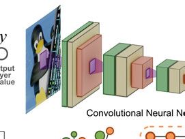
Forests (RF)[29] and convolutional neural networks (CNN). In recent years,
one of the most used CNN architectures for nuclei detection is the U-net
architecture [30] and derived architectures like Tiramisu [31]. Figure 4.1 in
the next chapter shows a basic architecture of a CNN.
Objects can be detected by their contours. Contour or edge detection
algorithms [32] include Laplacian of Gaussian (LoG), Canny edge detection,
Sobel and Prewitt filters. Once borders are detected, closed or nearly closed
borders can be filled and connected components can be considered objects. If
the object intensities in the image do not vary greatly, thresholding can also
be a way to binarize an image and connected components of specific sizes
can be deemed objects.
Watershed algorithms, conceptually, treat the image intensities as a
landscape, which when filled with water would create “puddles” that
correspond to connected components which can be object candidates. Local
minima are treated as locations where water can spring and start filling up the
valley. For paper IV we use nuclei objects segmented using watershed as
implemented in the popular digital pathology software QuPath [33].
Machine learning methods for object detection perform a study of the
pixels under given labels and create a classifier that indicates whether a pixel
belongs to a specific object or to background. The most commonly used
method which is included as an option in most of the clinically used software
[34, 33] is RF, which takes as input many features coming from each pixel
and its neighboring pixels, mainly intensity, edge and textures. Such features
23serve to characterize a pixel as belonging to a particular class and RFs are able to distinguish them, resulting in the separation of objects’ pixels from background. Texture descriptors which are still commonly used in this area are, Gabor filters, edge filter, and filters in the frequency domain like filtering by band, Haan windows and wavelet filters. Classical image analysis methods applied to microscopy are reviewed here [12]. More modern methods like CNNs (described in more detail in chapter 4) learn their own unique features that allow them to classify and separate the pixels. The inputs are small portions of the images referred to as patches, which undergo a series of convolutions with matrices that contain the features. These features change as the network learns by means of back-propagating errors using gradient descent. 3.2.2 Region segmentation Segmentation is not only used to find objects, but also bigger regions of interest. The search for such regions focuses on texture instead of the shape of a particular object. All the methods explained previously, apply for region segmentation. In microscopy, image segmentation is, for example, focused on separating regions of diseased tissue from healthy tissue, or finding the boundary between them. It is also used to find specific types of tissue and distinguish them by the organ or location they come from. If a whole image contains a single region, textures measures can serve as a features to classify the image as belonging to a single class and separating it from other images in a dataset. In paper II we used image segmentation to distinguish cancer regions and quantify only within such regions. 3.3 Image registration Images of a single sample can be taken in different modalities, or the same modality but at different times and conditions. Sometimes, in order to create a large image in high resolution it is necessary to obtain smaller overlapping fields of view that need to be stitched together. In any case, multiple views of a sample can contribute to additional information and they need to be brought to the same spatial frame of reference. The process of aligning images is called image registration. Its specific use in medical images is surveyed in [35]. The transformation can have various degrees of freedom. The simplest one is called rigid, when it only requires translation, rotation and isotropic scaling (same scaling in all dimensions), such transformations preserve distances within the image and preserve parallel lines. When more distortion is required such as shear, the transformation is called affine, it preserves parallel lines but does not necessarily preserve distances. When the deformation goes in different directions and magnitudes along the image the registration 24
transformation is called deformable/elastic/non-rigid and the most commonly
used kind is B-spline [36, 37].
   Image registration is expressed as an optimization problem that is solved by
iteratively searching for the parameters θ of a transformation T that transforms
an image A (moving) into the reference space of image B (fixed). The best
alignment is decided based on a distance measure d between the reference
image and the moving image. Registration can then be defined as:
                             arg min d(T (A, θ ), B)                       (3.1)
                                θ
   Image registration can be feature based or intensity based. Feature based
means that several matching points have to be found in the images and then a
transformation that is able to minimize the distance between these points.
Intensity based methods use pixel intensities to guide the registration. There
are a few kinds that include both features and intensities, such as [38] which
is used in paper II to find affine transformations between cores in a TMA.
Using a single transformation for a whole image does not take into account
possible disconnected objects of interest that move and transform
independently. In such case, piecewise transformations can be used, this can
be useful for very large image such as those in microscopy. In paper III the
size of image, the disconnected pieces and the image artifacts called for a
piecewise affine registration using feature based registration. While features
can be any of the ones presented in previous chapters, in this case features
invariant to scale called SIFT [39] were used to find the parameters of the
affine transformation.

3.4 Color transformation and unmixing
The colors we see in images in computer screens are usually the combination
of several grayscale channels. The most commonly known one is RGB
(red,green,blue). Most color images are stored in such an RGB format. When
we open the image using a viewer the channels are combined and the result
are many different hues. As seen in previous chapters microscopy images
come from brightfield and fluorescence microscopy and the colors they have
vary depending on the scanner, the stain, the camera settings and many more
factors.
   When a method is designed to work for a particular colored dataset, it
seldom works on different colored data if unchanged. For this reason, it is
desirable to transform the color of the images into a common space where a
single method can work. This can be done with methods as simple as linear
transformation of the color channels or with complex deep learning tools like
generative adversarial networks (GAN) and U-Net architectures [40, 41].
   To extract a color from an image, i.e. separate stains into channels other
than RGB, say, H&E or HDAB, it is necessary to know a color base. Since

                                                                             25
Figure 3.2. Examples of registration. Affine matrices contain 9 values in 2D out of which 6 represent a linear transformation of the X and Y coordinates. Affine transformations preserve parallel lines as observed in the squares surrounding the tissue. B-spline transformations require a set of control points and knot points. Piece- wise affine transformations require the polygon around the piece and its corresponding affine transformation matrix. RGB is a 3 channel color then a 3D base can be found from a reference image in which 3 vectors can separate the image into 3 channels different from RGB that are a linear combination of them. We use color transformations to transform RGB colored images to HDAB in papers III and II. 3.5 Open source software tools for image analysis This is a short section where I describe the libraries and software that are building blocks in image analysis and that are close to the mathematical models that will be discussed in the thesis. While there is many software out there built as a tool for the use of image analysis for the general public, I will mention the key players that still to this day continue to develop methods and 26
make them available through their libraries and software under open source
licences.
   In 2007, when I started my journey in image analysis I was introduced to
C++ programming language for image analysis and computer graphics. The
python programming language was still not big in image or data analysis.
Mainly the open source software for image analysis I was aware of in C++
was ITK [42] which started in 1999 but was released in 2002. It is still widely
used and is the backbone of specialized image processing libraries. At the
same time, at Intel Research, the Open Computer Vision (OpenCV) [43]
library was formed. In 2003 based on ITK, Elastix[44] introduced a general
framework for image registration.
   More specialized libraries and software for microscopy start to be built.
Joining the race since 1997, the National Instutes of Health (NIH) provide
grants to different groups work on C++ and Java to create an image analysis
software that would become ImageJ [45] and FIJI [46] which is one of the most
popular software for image analysis in life sciences. The NIH also develops
Bio-Formats+[18] which come out 2006.
   Using C and C++ under the hood, building on work in numerical methods
and a library, the library Numpy [47] comes to the world in 2006 making it
easier to work with multidimensional arrays such as images. The now
ubiquitous python’s scikit-learn (2007) [48] and scikit-image (2009) [49]
come to the world for scientific machine learning and image processing.
Bindings in python for OpenCV and Elastix are developed.
   In 2005 CellProfiler [50] by the Broad Institute comes out and is specially
designed for quantitative microscopy image analysis. In 2008 CellProfiler
Analyst [51] comes out for the use of more advances machine learning
methods for cells classification. For segmentation, in 2011, Ilastik [52] offers
machine learning methods such as random forests to perform image
segmentation with an interactive GUI.
   With the improved computational power deep learning came back into the
mix and libraries like Torch are ported into python creating Pytorch [53] in
2016, and while it is a machine learning library it contains its own matrix
representation, tensors. In 2018 pytorch-geometric [54] comes out for working
with deep learning for graphs.
   I can’t possibly name all the software that I have encountered during this
research but I consider these to be corner stones for image analysis and it’s
use in microscopy (not exclusively). There is software more interested in the
application of methods rather than on the development, so it’s not mentioned
in this section but rather in context in the next sections.

                                                                            27
4. Quantitative Data Analysis To gain understanding on a phenomenon we measure and collect data, be it numerical or pictorial. Any kind of measurement includes noise, so data is first cleaned, or denoised. Then it can be inspected in an exploratory phase where statistical modelling can be of use. It helps to understand the scope, the range in which data is present. Data can be used not only for exploration but also for analysis and prediction. Models can be created from the data and their errors can be assessed so that the best available models can be used to associate features to specific points. These models can offer insights as to what characterizes the data and allows us to separate it into different and useful categories. The models can also be used to predict new information and to make decisions. One of the most important uses of data analysis today is the combination of multiple sources of information. It is often not enough to analyze a single source but to bring information of multiple experiments designed in different ways and performed at different times under different conditions and producing different kinds of output. During the research leading to this thesis, data was extracted from microscopy images so that tissues and cells could be characterized. The data was analyzed so that tissues could be assigned, for example, an origin, a grade, an amount of cells, an amount of pixels and more. Cell can have several features computed, such as size, intensities, textures, classes and more. All this information can come from different sources, such as different images and from expert observations, such as those from pathologists. Observations from experts can be used as labels for further processing by e.g. machine learning. 4.1 Classification Given a set of observations with a set of features and an associated label, we want to learn how to separate them into categories so that a new observation can be given a label corresponding to one such category based on the features associated to it. For example, is it a cancer cell or not? or which cell type does a cell resemble? is it a neuron or is it a macrophage? Can I discriminate (distinguish) them with the information I have or do I have to collect more information and use more sources? This type of problem is called supervised learning. 28
Classification produces a function (or model) that assigns a category to an
input commonly described by a vector which contains independent variables,
called the feature vector. In a probabilistic setting, the model can also assign
probabilities instead of a single class prediction. To train a classifier, a set of
training data with labels for each of the observation should be available. The
most basic model, which also serves as a building block in more advanced
models for classification, is a linear model for binary classification (meaning
belonging to a class or not). In a linear model a prediction ŷ is found from
feature vector input x of length n and a weighted linear combination of its
components. The weights, or parameters θ is what we want to find. A binary
linear classifier can be expressed as
                                         n
                                  ŷ =   ∑ θ jx j.                          (4.1)
                                         j=1

To find θ , the classification problem is posed as an optimization problem with
an objective function J
                             J(θ ) = L(θ ) + Ω(θ ),                         (4.2)
where L is a loss function and Ω is a regularization function. The loss
measures how similar the predicted labels are to the original labels, while the
regularization function, as its name suggests, regulates the values for θ by
penalizing the appearance of undesired properties to try to avoid overfitting to
a particular dataset.
   However if we look closely at equation 4.1 what the model is doing is not
yet exactly classification[55], but regression. We are approximating the values
of y. This means that if our labels are a vector of 0 and 1, ŷ will still be
penalized if it is far away despite being in the right direction, for example
having predicted a 3 instead of a 1 or a -2 instead of a 0. To find the final class
prediction one can threshold ŷ at 12 .

4.2 Unsupervised learning
4.2.1 Clustering
When there are no available labels for a dataset, it can still be separated into
classes by clustering, which is a type of unsupervised (without labels)
learning. Clustering works on the basis of dividing observations into groups
that share similar features, or even groups them by the neighbors that an
observation has rather than its inherent features. Clustering will also yield a
model so that any new input can be assigned a class based on its similarity to
the divisions found. A really good review and implementation of classical
methods for clustering is available in [56, 48] and a general overview can be
found in [57].

                                                                               29
There is no one-size-fits-all clustering method. There are methods that
require as a parameter the number of clusters and others that attempt to
discover the number of clusters. Additionally, every method makes
assumptions about the data. If data is not distributed according to the
assumptions, the model will behave unexpectedly. Since clustering is based
on the similarity between observations, this similarity can be almost any
pairwise distance measure. Usual measures are euclidean and cosine, it
depends on the manifold the data lies on.
The most common clustering method that requires specifying the number
of clusters is k-means. Its goal is to divide a set of observations into k separate
clusters C characterized by their centroids. K-means minimizes the euclidean
distances from every observation to each cluster in C. The observation will be
assigned the label of the cluster whose mean it is closest to.
n 2
∑ min (xi − μ j ) (4.3)
i=0 μ j ∈C
But then again, k-means makes assumptions of data, any clustering based
on k-means will result in a partition that is equivalent to a voronoi partition
which is convex and therefore restricts the resulting shapes of clusters. This
may often be ill-suited for actual data, which is why less restrictive methods
have been devised.
Another type of clustering methods create a tree that iteratively splits the
dataset into smaller subsets until each subset consists of only one observation
[58]. The tree can either be created from the leaves up to the root
(agglomerative) or from the root down (divisive) by merging or dividing
clusters at each step. These methods require in most cases a stopping
criterion which become another parameter.
Density-Based Spatial Clustering of Applications with Noise (DBSCAN)
[59] finds observations of high density and expands clusters from them. It was
one of the first clustering methods based on density and is resistant to noise.
DBSCAN is insensitive to the shape of the cluster but is sensitive to the density
variation.
Mode-seeking methods estimate the density of all the observations and
then identify the local density maxima which become candidates for centers
of clusters. The most common method in this category is called mean-shift
[60], which iteratively searches the neighborhood around candidates to
cluster centers and computes a vector m that is the difference between the
weighted mean of values within a kernel and the center of such kernel. This
vector m is the mean shift vector, which goes in the direction of a region with
a higher density of observations.
Clustering can be done in several data representations, be it an image or a
graph. When objects like cells (or objects inside cells) have a spatial location
and distances to neighbors can be quantified, the objects can be represented
by a graph G with nodes V and edges E. Edges are only formed when two
30You can also read