Imaging a photodynamic therapy photosensitizer invivo with a time-gated fluorescence tomography system
←
→
Page content transcription
If your browser does not render page correctly, please read the page content below
Imaging a photodynamic therapy
                 photosensitizer in vivo with a time-gated
                 fluorescence tomography system

                 Weirong Mo
                 Daniel Rohrbach
                 Ulas Sunar

Downloaded From: https://www.spiedigitallibrary.org/journals/Journal-of-Biomedical-Optics on 23 Feb 2021
Terms of Use: https://www.spiedigitallibrary.org/terms-of-use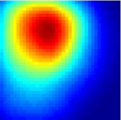
Journal of Biomedical Optics 17(7), 071306 (July 2012)

                Imaging a photodynamic therapy photosensitizer in vivo
                with a time-gated fluorescence tomography system
                Weirong Mo, Daniel Rohrbach, and Ulas Sunar
                Roswell Park Cancer Institute, Department of Cell Stress Biology and PDT Center, Elm and Carlton Streets, Buffalo, New York, 14263

                              Abstract. We report the tomographic imaging of a photodynamic therapy (PDT) photosensitizer, 2-(1-hexyloxyethyl)-
                              2-devinyl pyropheophorbide-a (HPPH) in vivo with time-domain fluorescence diffuse optical tomography
                              (TD-FDOT). Simultaneous reconstruction of fluorescence yield and lifetime of HPPH was performed before
                              and after PDT. The methodology was validated in phantom experiments, and depth-resolved in vivo imaging
                              was achieved through simultaneous three-dimensional (3-D) mappings of fluorescence yield and lifetime contrasts.
                              The tomographic images of a human head-and-neck xenograft in a mouse confirmed the preferential uptake
                              and retention of HPPH by the tumor 24-h post-injection. HPPH-mediated PDT induced significant changes in
                              fluorescence yield and lifetime. This pilot study demonstrates that TD-FDOT may be a good imaging modality for
                              assessing photosensitizer distributions in deep tissue during PDT monitoring. © 2012 Society of Photo-Optical Instrumentation
                              Engineers (SPIE). [DOI: 10.1117/1.JBO.17.7.071306]

                              Keywords: fluorescence; diffusion; tomography; imaging system; image reconstruction; photodynamic therapy.
                              Paper 11602SS received Oct. 14, 2011; revised manuscript received Feb. 20, 2012; accepted for publication Mar. 5, 2012; published
                              online May 16, 2012.

                1     Introduction                                                                 contrast: fluorescence lifetime.14,42–48 As an intrinsic property of
                Photodynamic therapy (PDT) is a clinically attractive treatment                    a fluorophore, the fluorescence lifetime is independent of fluor-
                                                                                                   escence signal intensity, allowing time domain to be a robust
                option for eradicating early-stage cancers.1–3 With high tumor
                                                                                                   technique for tumor demarcation.35,49–53 Fluorescence lifetime
                avidity, the chlorin-based compound 2-(1-hexyloxyethyl)-2-
                                                                                                   may change in response to local molecular and cellular changes
                devinyl pyropheophorbide-a (HPPH) has been shown to be a
                                                                                                   such as binding, polarity, pH value, and oxygenation sta-
                potential photosenstizer for imaging and treatment.4 Recent
                                                                                                   tus.34,54,55 As such, changes in fluorophore lifetime can be
                HPPH-oriented laboratory research and early-phase clinical stu-
                                                                                                   potential noninvasive biomarkers for investigating and visualiz-
                dies at Roswell Park Cancer Institute (RPCI) have demonstrated
                                                                                                   ing the local microvascular changes, photophysical processes,
                that HPPH-mediated PDT is an effective treatment option for                        and photochemical reactions at molecular and cellular
                superficial cancers such as skin and head and neck lesions in                      levels.55–59 For example, microscopic TD imaging has been
                the oral cavity.4–8                                                                applied for studying photobleaching and lifetime dynamics of
                    The efficacy of PDT is largely dependent on the spatial                        PDT photosensitizers in cells.55,56,60,61
                distribution and temporal changes of the photosensitizer.9–11                          In this paper, we report the application of TD-FDOT for 3-D
                Fluorescence properties of photosensitizers can be utilized to                     reconstructions of the fluorescence yield and lifetime of the
                assess the photosensitizer content. Due to its simplicity, fluor-                  photosensitizer HPPH in vivo before and after PDT. We first
                escence spectroscopy has been employed in many preclinical                         describe a TD-FDOT system, which employs an ultra-short
                and clinical studies (see reviews in Refs. 9 and 12). However,                     pulse laser, gated imaging, and time-delay techniques. We
                fluorescence spectroscopy is not well suited for quantifying spa-                  demonstrate the performance of the imaging system in resolving
                tial heterogeneities of optical properties, especially when deeper                 the fluorescence yield and lifetime of HPPH with phantom
                and thicker tissue is being investigated. In recent years, nonin-                  experiments. Then we show in vivo mouse imaging results.
                vasive near-infrared fluorescence diffuse optical tomography                       Further, we quantify the changes in these parameters due to
                (FDOT) technologies emerged as viable approaches for imaging                       PDT. Our imaging results show that the HPPH preferentially
                heterogeneities in deep tissue. For example, FDOT has been uti-                    accumulated in the tumor, which allowed accurate localization
                lized as quantitative imaging for the localization of fluorophores                 of the tumor. In addition we show depth-resolved photobleaching
                in deeply seated tumors, as well as for therapy monitoring.13–32                   and lifetime changes due to HPPH-mediated PDT. This study
                    Among FDOT modalities, the time-domain (TD) modality                           demonstrates the utility of the TD-FDOT system for monitoring
                provides superior sensitivity over continuous-wave FDOT and                        PDT with fluorescence yield and lifetime contrasts.
                frequency-domain FDOT for detecting weak fluorescence sig-
                nals.33–35 It can quantify absolute concentration and depth of                     2       Methods
                a fluorophore by analyzing time-of-flight measurements.36–41
                In addition, TD-FDOT offers quantification of another imaging                      2.1      Experimental TD-FDOT System
                                                                                                   Figure 1 shows the schematic of our experimental TD-FDOT
                Address all correspondence to: Ulas Sunar, Roswell Park Cancer Institute,          system. Planar transmission geometry was adopted to achieve
                Department of Cell Stress Biology and PDT Center, Elm and Carlton Streets,
                Buffalo, New York, 14263; Tel.: +1 7168453311; Fax: +1 7168458920;
                E-mail: ulas.sunar@roswellpark.org                                                 0091-3286/2012/$25.00 © 2012 SPIE

                Journal of Biomedical Optics                                              071306-1                                               July 2012   •   Vol. 17(7)

Downloaded From: https://www.spiedigitallibrary.org/journals/Journal-of-Biomedical-Optics on 23 Feb 2021
Terms of Use: https://www.spiedigitallibrary.org/terms-of-use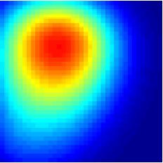
Mo, Rohrbach, and Sunar: Imaging a photodynamic therapy photosensitizer : : :
Y
Z Mouse and Chamber 2.2 Data Acquisition
XY
X Filter
Mirror Steering In order to acquire the time-resolved signals, the “comb” mode
Galvo Image
Intensifier
CCD of the image intensifier was utilized. The gate width Δτgate was
Lens set to be 0.8 ns. The delay of the temporal acquisition,
DAQmx
Tank Lens τdelay ¼ N · Δτdelay , N ¼ ½1 : : : N d was set to be τdelay ¼
(PCI-6259)
BPF or OD
Wf Wr ½0; 0.8; 1.6; : : : ; 12 ns, where the incremental step Δτdelay ¼
Filter Tx / Rx
Computer 0.8 ns and N d is the number of delay steps. The bias voltage
Sync. Delayed Delayed of the image intensifier V bias (configurable in ½200 : : : 850 V)
Pulsed Trigger Trigger Trigger HR Image
Intensifier
Trigger was fixed at 670 V and the exposure time of the CCD, τexp
laser Delay Unit Controller
was optimized to avoid signal saturations. These system settings
Electrical signal Light path Tumor on mouse are similar to previous work42,62,63 and were optimized empiri-
cally with considerations of CCD’s dynamic range, gain of
Fig. 1 Schematic of time-domain fluorescence diffuse optical tomogra- the image intensifier, dark noise, HPPH dose and lifetime,
phy (TD-FDOT) system. and the data-acquisition time. In addition, the images acquired
by the CCD camera binned to 128 × 128 pixels to increase the
large-area tissue sampling with the combination of a galvan- signal-to-noise ratio.
For each imaging experiment, three types of data sets
ometer scanner and a lens coupled charge-coupled device
were acquired: intrinsic excitation, fluorescence emission, and
(CCD) camera.15,16,42 A 660 nm pulsed laser (BHLP-660,
leakage. The data set of intrinsic laser excitation φex , which
Becker & Hickl GmbH) was used as the light source to
characterizes the system response in the presence of the imaging
match HPPH’s absorption peak at 665 nm.5 The laser has a
objects, was acquired by mounting a neutral-density filter (OD2)
pulse repetition rate of 50 MHz. The average optical power
in front of the image intensifier. The data set of fluorescence
was set to ∼0.5 mW, and the full-width-at-half-maximum
emission φem was acquired in a similar way, but by replacing
(FWHM) of the laser pulse was ∼120 ps. The spectrum of
the OD2 filter with a 720 nm bandpass fluorescence filter.
the collimated laser beam was first corrected with a bandpass
The data set of leakage signal φlk , which accounted for the
filter (BPF) in front of the laser, and then the laser beam was
bleeding-through of excitation light through the fluorescence
focused on the front wall of the imaging chamber (W f in
filter, was acquired in a similar way as fluorescence emission,
Fig. 1). The imaging chamber was sandwiched between two but with no fluorescence object in the imaging chamber.16,42,64,65
pieces of transparent, antireflection-coated glass, allowing an The exposure time τexp was 400 ms during excitation, emission,
imaging volume of 80 mm × 80 mm × 18 mm. Homogenous and leakage measurements. Figure 2 shows an example of a
optical matching fluid, prepared by mixing India ink, Intralipid time-resolved excitation and emission data from a HPPH
suspension, and water, was poured into the tank to serve as the phantom experiment. The leakage signal was negligible
homogeneous image background for phantom and mice experi- (mean standard deviation of φlk was less than 2% of mean
ments. The emission signals from the rear wall (W r in Fig. 1) deviation of φem , data not shown) under these experimental
sequentially passed through an optical filter, a collimation lens settings and optical properties.
set (AF NIKKOR 50 mm f/1.4D, Nikon), and a high-gain image
intensifier (PicoStar HR-12, LaVision) and was captured by a
highly sensitive CCD camera (12 bit, Imager QE, LaVision). 2.3 Image Reconstruction
The high-gain image intensifier worked in a time-gated, or a
“comb” mode, as described previously.42 Briefly, each laser The quantification of fluorescence yield and lifetime was based
pulse (pulse rate ¼ 50 MHz) synchronously produced a trigger on the normalized Born approximation.13,15,17,64 By making use
signal, which served as a timing reference. This trigger opened a of self-calibrated data that divide the fluorescence measure-
ments with corresponding excitation measurements, the normal-
high-rate image intensifier (HRI) gate after a fixed time delays.
ized Born ratio works with analytical or numerical forward
Time delays can be set by a delay unit, and gate widths can be
solvers and offers significant experimental advantages as it
set by HRI. The intensifier boosts the signal originated from the
is independent of source strengths, detector gains, coupling
object. The CCD camera collected the boosted optical signal and
efficiency to tissue. These advantages significantly simplify
streams data into personal computer. The CCD camera exposure
the image reconstruction.16,17,64,66 Such image reconstruc-
length determines the number of laser pulses that are integrated.
tion method was recently reported to resolve 50 ps lifetime
As the pulsed laser had a repetition rate of 50 MHz, 5 × 10⁷
changes with a similar instrumentation approach.42 The acquired
images could be accumulated if the CCD acquisition time
was 1 s. As the trigger signals were delayed incrementally, 1 Excitation
Intensity (Norm)
the combination of image intensifier and CCD camera can Emission
record a sequence of images, which reflects the time-resolved
photon intensity. An ultra-sharp, narrow bandpass filter 0.5
(FF01-720/13-25, Semrock) in front of the image intensifier
rejected undesired excitation photons. The incident laser
beam was steered in an XY raster pattern by a high-quality pro- 0
grammable galvanometer scanner (ProSeries-10, Cambridge 0 5 10
time (ns)
Technology). The entire experimental system was automated
under computer control through a data acquisition module Fig. 2 Temporal profiles (normalized) obtained from HPPH experiment.
(NI-DAQmx, PCI-6259, National Instruments) and a custom (Red circle line): Fluorescence emission and (blue triangle line): Laser
LabVIEW (Version 8.5, National Instruments) program. excitations.
Journal of Biomedical Optics 071306-2 July 2012 • Vol. 17(7)
Downloaded From: https://www.spiedigitallibrary.org/journals/Journal-of-Biomedical-Optics on 23 Feb 2021
Terms of Use: https://www.spiedigitallibrary.org/terms-of-use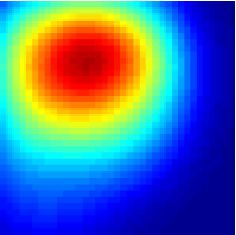
Mo, Rohrbach, and Sunar: Imaging a photodynamic therapy photosensitizer : : :
time-resolved data were first converted into frequency domain. ImðXk Þ
The real and imaginary information were extracted for resol- Xk by τk ¼ and
ω · ReðXk Þ
ving the fluorescence yield and lifetime simultaneously. Any
harmonic frequencies ranging from base frequency f base ηk ¼ ReðXk Þ þ ω · τk · ImðXk Þ.
through maximum frequency f max ¼ N · f base can be utilized
for image reconstruction, where integer N is the order of
harmonics or the total time-delay steps.42,45 For example, in the 2.4 Phantom and In Vivo Imaging
settings of HPPH experiments, 16 time-resolved images were
acquired sequentially for a given time-step size of 0.8 ns. The The laser scanning pattern was set to be an 8 × 8 grid, giving a
information at fundamental frequency is thus, f base ¼ total of 64 source positions (blue “þ” in Fig. 3). The laser beam
½1∕16 samples∕ð0.8 ns∕sampleÞ ¼ 78.125 Mhz and f max ¼ had a diameter of ∼0.3 mm when focused on the imaging tank
16 · f base ¼ 1.25 GHz. For the results reported here, we used and was assumed to be a point source. The point-to-point
the fundamental frequency f base for the image reconstruc- separation was 3 mm, giving a total scanning area of
tion. A MATLAB (R2009a, The MathWorks, Inc.) program ∼24 mm × 24 mm. For mouse imaging, this scanning area
was constructed to solve the discrete linear equation ΦnB ¼ could cover the tumor with some peripheral tissue. On the detec-
W · X, where tion plane (Z ¼ 18 mm), we chose 64 pixels, which had
identical X and Y positions as 64 source positions (red “circle”
ΦnB ½rsðiÞ ; rdðjÞ ; ω in Fig. 2). Each pixel, having a spatial area of ∼0.4 mm ×
0.4 mm, was assumed as an infinitesimal point detector. In
Φem ½rsðiÞ ; rdðjÞ ; ω; λem − Φlk ½rsðiÞ ; rdðjÞ ; ω; λex (1)
¼ ; total 4096 source-to-detector measurements were selected. At
Φex ½rsðiÞ ; rdðjÞ ; ω; λex each laser source position, 15 consecutive temporal images
(N d ¼ 15) were acquired with an increasing temporal interval
Wði;j∶kÞ ¼ −S0 of Δτdelay ¼ 0.8 ns, giving a temporal length of 12 ns.
Phantom experiments were conducted prior to the mouse
Gsv ½rsðiÞ ; rvðkÞ ; ω; λex · Gvd ½rvðkÞ ; rdðjÞ ; ω; λem experiments. The optical matching fluid with absorption co-
· ;
Gsd ½rsðiÞ ; rdðjÞ ; ω; λex efficient μa ¼ 0.4 cm−1 and reduced scattering coefficient μs0 ¼
10.0 cm−1 was filled into the imaging tank to mimic the optical
(2)
properties of healthy mouse tissue. The absorption and reduced
scattering coefficients were assumed to be similar at excitation
ηk · μem
a
Xk ¼ : (3) and emission wavelengths. Hence these two parameters were
1 − iωτk substituted into the normalized Born ratio as fixed values. A
transparent plastic tube (diameter ¼ 5 mm), containing HPPH
Here ΦnB ½rsðiÞ ; rdðjÞ ; ω is the normalized Born ratio of emis- fluorophore (concentration ¼ 0.5 μM) in identical matching
sion photon density to excitation photon density. The weight fluid, was inserted into the tank vertically at the position
matrix Wði;j∶kÞ accounts for the perturbation of fluorescence het- ðX; ZÞ ≈ ð−4.0; 9.0Þ mm to mimic the tumor heterogeneity.
erogeneities at voxel vðkÞ in response to the excitation at source In order to characterize the accuracy of the image reconstruc-
position rsðiÞ and the emission at the detector position rdðjÞ . tion, especially the fluorophore’s lifetime, we conducted another
Φem ½rsðiÞ ; rdðjÞ ; ω and Φex ½rsðiÞ ; rdðjÞ ; ω are temporal point- phantom experiment using a well-known fluorescence com-
spread functions (TPSF) of emission φem ½rsðiÞ ; rdðjÞ and excita- pound, Atto655 (93711, Sigma-Aldrich). We chose Atto655
tion φex ½r sðiÞ ; r dðjÞ in Fourier domain, respectively. λem and λex because it has similar excitation and emission peaks (λex ¼
are excitation wavelength and the emission wavelength, 665 nm, λem ¼ 690 nm) and the same order of magnitude life-
respectively. ω ¼ 2πf base is the fundamental angular frequency, time (1.9 ns in water), which allowed using similar experimental
which can be determined by the temporal sampling interval of settings. The tube containing Atto655 (concentration ¼ 0.5 μM)
the experiment. G is a two-point Green’s function in frequency in optical matching fluid was placed vertically on the
domain,42,45 with an altered form in order to account for the slab position ðX; ZÞ ≈ ð4.0; 9.0Þ mm.
boundary conditions,67 S0 is a calibration factor depending on
the geometry and optical properties.17 The unknown volumetric
variable Xk , which encompasses spatial variations of fluores- Compound
cence yield ηk and lifetime τk , can be resolved by inverting
the linear equation ΦnB ¼ W · X. As a straightforward solution 20
Sources
to this linear equation, in which complex numbers involved, Detectors
terms of ΦnB , W, and X are decomposed and rewritten as
Y [mm]
0
ReðΦnB Þ ReðWÞ −ImðWÞ ReðXÞ
¼ · ;
ImðΦnB Þ ImðWÞ ReðWÞ ImðXÞ -20
20
20
Wr 10
where Reð·Þ and Imð·Þ stands for real and imaginary parts of the 0
corresponding quantities, respectively. In this study, the alge- Z [mm] 0 -20
X [mm]
braic reconstruction technique (ART) was used to iteratively Wf
resolve Xk and reconstruct images for both phantom and Fig. 3 Illustration of transmission geometry. Blue “þ”: laser scanning
mouse data.68 The 3-D mappings of fluorescence yield and positions on the source plane (W f , Z ¼ 0 mm). Red “•”: detector posi-
lifetime can be achieved simultaneously by rearranging the tions on the detection plane (W r , Z ¼ 18 mm). The 64 detectors have
volumetric vector identical X-Y positions as 64 source positions.
Journal of Biomedical Optics 071306-3 July 2012 • Vol. 17(7)
Downloaded From: https://www.spiedigitallibrary.org/journals/Journal-of-Biomedical-Optics on 23 Feb 2021
Terms of Use: https://www.spiedigitallibrary.org/terms-of-use
Mo, Rohrbach, and Sunar: Imaging a photodynamic therapy photosensitizer : : :
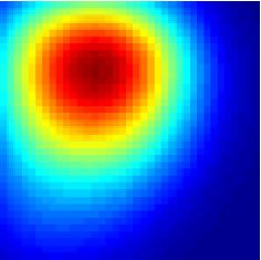
Z = 1 mm Z = 5 mm Z = 9 mm Z = 13 mm Z = 17 mm
(B) 10 10 10 10 10 1
Yield [a.u]
5 5 5 5 5
HPPH (A)
Y [mm]
Y [mm]
Y [mm]
Y [mm]
Y [mm]
20 0 0 0 0 0 0.5
10 -5 -5 -5 -5 -5
Y [mm]
0 -10 -10 -10 -10 -10 0
-10 0 10 -10 0 10 -10 0 10 -10 0 10 -10 0 10
X [mm] X [mm] X [mm] X [mm] X [mm]
-10 10 10 10 10 10 6
Lifetime [ns]
-20 5 5 5 5 5
Y [mm]
Y [mm]
Y [mm]
Y [mm]
Y [mm]
4
-30 0 0 0 0 0
-20 0 20
-5 -5 -5 -5 -5 2
X [mm]
-10 -10 -10 -10 -10 0
-10 0 10 -10 0 10 -10 0 10 -10 0 10 -10 0 10
X [mm] X [mm] X [mm] X [mm] X [mm]
(D) Z = 1 mm Z = 5 mm Z = 9 mm Z = 13 mm Z = 17 mm 1
10 10 10 10 10
5 5 5 5 5
Yield [a.u]
Atto655 (C)
Y [mm]
Y [mm]
Y [mm]
Y [mm]
Y [mm]
20 0 0 0 0 0 0.5
10 -5 -5 -5 -5 -5
Y [mm]
0 -10 -10 -10 -10 -10 0
-10 0 10 -10 0 10 -10 0 10 -10 0 10 -10 0 10
X [mm] X [mm] X [mm] X [mm] X [mm]
-10 10 10 10 10 10 2
Lifetime [ns]
-20 5 5 5 5 5 1.5
Y [mm]
Y [mm]
Y [mm]
Y [mm]
Y [mm]
-30 0 0 0 0 0 1
-20 0 20
X [mm] -5 -5 -5 -5 -5 0.5
-10 -10 -10 -10 -10 0
-10 0 10 -10 0 10 -10 0 10 -10 0 10 -10 0 10
X [mm] X [mm] X [mm] X [mm] X [mm]
Fig. 4 (a) Picture of phantom tube containing HPPH. White square shows the region of laser scanning and image reconstruction. (b) Reconstructed
images of fluorescence yield (top, unit: a.u) and lifetime (bottom, unit: ns) of HPPH at 5 different depths Z ¼ ð1; 5; 9; 13; 17Þ mm. (c) Picture of phantom
tube containing Atto655. White square shows the region of laser scanning and image reconstruction. (d) Reconstructed images of fluorescence yield
(top, unit: a.u) and lifetime (bottom, unit: ns) of Atto655 at five difference depths Z ¼ ð1; 5; 9; 13; 17Þ mm.
The in vivo mouse imaging and PDT treatments in this study imaging scan took ∼12 min. During the entire imaging and treat-
were performed in compliance with Roswell Park Cancer ment period, the mouse was kept anesthetized.
Institute Animal Study Committees’ requirements. A male
severe combined immunodeficiency (SCID) mouse (12 weeks 3 Results and Discussion
old, weight 30 grams) was inoculated subcutaneously with
human head and neck tumor tissue obtained from a patient dur- 3.1 Phantom Imaging
ing an ongoing clinical trial.7 The tumor was planted on the right
Figure 4(a) and 4(c) show the photographic pictures of HPPH
lateral flank of the mouse and grew up to a diameter of approxi-
and Atto655 phantom tubes and imaging area (white squares),
mately 10 mm (Fig. 4). The photosensitizer HPPH (3 μmol∕kg)
while Fig. 4(b) and 4(d) show how the corresponding image
was injected intravenously via tail vein 24-h before the imag-
reconstruction results in terms of fluorescence yield (top,
ing experiment and PDT treatment. To minimize motion
unit: a.u) and lifetime (bottom, unit: ns), respectively. For
artifacts during scanning, the mouse was anesthetized with
tomographic image reconstruction, the imaging chamber (slab
ketamine (100 mg∕kg), xylazine (10 mg∕kg), and aceproma-
thickness, total depth ¼ 18 mm) was evenly divided into five
zine (3 mg∕kg). The anesthetized mouse was secured in a holder non-overlapping slices, spanning from depth Z 1 ¼ 1.0 mm
to minimize motion and discomfort. The holder with the mouse through depth Z 5 ¼ 17.0 mm with a depth increment of 4 mm.
was submerged into the matching fluid-filled tank. The optical X and Y coronal images were reconstructed at these five depths.
properties of the matching fluid were identical to those of the After image reconstruction, for the lifetime quantification we
matching fluid made for phantom experiments. The temperature demarcated the object size by including any voxel with yield
of the matching fluid was kept around 35°C to prevent loss of values of at least 30% of the maximum yield.45 Based on
body heat. The mouse’s head was above the fluid for normal the thresholded lifetime images, the mean lifetime within
breathing and the mouse’s eyes were lubricated with tear gel the HPPH target area is found to be ð6.39 0.11Þ ns
to avoid drying. (mean standard deviation), which is within the range of pub-
During the PDT laser treatment, the mouse remained in lished results.69 From the HPPH images, the position of the tube
the imaging chamber while the optical matching fluid was axis was found to be ðX; ZÞ ¼ ð−4.0 0.5; 9.0 0.5Þ mm,
removed. The tumor area plus a small peripheral margin which agrees with the real center position ðX; ZÞ ¼ ð−4.0
(16 mm diameter spot size) was irradiated with 75 mW∕cm2 0.5; 9.0 0.5Þ mm. Moreover, the mean lifetime of Atto655
of 665 nm light from an Argon pumped dye laser. The treatment was found to be ð1.86 0.16Þ ns, which closely agrees with
took 10 min for a total dose of 45 Joules∕cm2 , and a single the standard value of 1.9 ns. Although we did not fully
Journal of Biomedical Optics 071306-4 July 2012 • Vol. 17(7)
Downloaded From: https://www.spiedigitallibrary.org/journals/Journal-of-Biomedical-Optics on 23 Feb 2021
Terms of Use: https://www.spiedigitallibrary.org/terms-of-use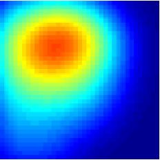
Mo, Rohrbach, and Sunar: Imaging a photodynamic therapy photosensitizer : : :
30 30
(A) (B) characterized the accuracy of our system in estimating lifetimes,
20 head 20 a recent study by Nothdurft et al.42 reported a 50 ps lifetime
10 10 sensitivity using a similar system and reconstruction strategy.
Y [mm]
Y [mm]
0 0
3.2 In Vivo Mouse Imaging
-10 -10
tail The mouse imaging was reconstructed in a similar way as the
-20 -20
phantom images. Figure 5(a) shows the picture of the mouse
-20 0 20 -20 0 20
outlined by white curves and tumor position pointed by red
X [mm] X [mm] arrow. Figure 5(b) shows the scanned and imaged tumor area
and surrounding peripheral normal tissues. The area in the
Fig. 5 (a) Picture of mouse outlined by white curves, and tumor position white square shows the laser scanning and image reconstruction
pointed by red arrow; (b) region of interested outlined by the white areas. The tumor area, indicated by the red circle, was located
square will be reconstructed. Red circle shows the tumor area.
approximately in the top-left quadrant. The same mouse was
Z = 1 mm Z = 5 mm Z = 9 mm Z = 13 mm Z = 17 mm
5 5 5 5 5 0.04
0 0 0 0 0 0.03
Yield [a.u]
Y [mm]
Y [mm]
Y [mm]
Y [mm]
Y [mm]
-5 -5 -5 -5 -5 0.02
-10 -10 -10 -10 -10 0.01
-15 -15 -15 -15 -15 0
-5 0 5 10 15 -5 0 5 10 15 -5 0 5 10 15 -5 0 5 10 15 -5 0 5 10 15
X [mm] X [mm] X [mm] X [mm] X [mm]
5 5 5 5 5 6
Lifetime [ns]
0 0 0 0 0
Y [mm]
Y [mm]
Y [mm]
Y [mm]
Y [mm]
4
-5 -5 -5 -5 -5
-10 -10 -10 -10 -10 2
-15 -15 -15 -15 -15 0
-5 0 5 10 15 -5 0 5 10 15 -5 0 5 10 15 -5 0 5 10 15 -5 0 5 10 15
X [mm] X [mm] X [mm] X [mm] X [mm]
Z = 1 mm Z = 5 mm Z = 9 mm Z = 13 mm Z = 17 mm 0.04
5 5 5 5 5
0 0 0 0 0 0.03
Yield [a.u]
Y [mm]
Y [mm]
Y [mm]
Y [mm]
Y [mm]
-5 -5 -5 -5 -5 0.02
-10 -10 -10 -10 -10 0.01
-15 -15 -15 -15 -15 0
-5 0 5 10 15 -5 0 5 10 15 -5 0 5 10 15 -5 0 5 10 15 -5 0 5 10 15
X [mm] X [mm] X [mm] X [mm] X [mm]
5 5 5 5 5 6
Lifetime [ns]
0 0 0 0 0
Y [mm]
Y [mm]
Y [mm]
Y [mm]
Y [mm]
4
-5 -5 -5 -5 -5
-10 -10 -10 -10 -10 2
-15 -15 -15 -15 -15 0
-5 0 5 10 15 -5 0 5 10 15 -5 0 5 10 15 -5 0 5 10 15 -5 0 5 10 15
X [mm] X [mm] X [mm] X [mm] X [mm]
Z = 1 mm Z = 5 mm Z = 9 mm Z = 13 mm Z = 17 mm 0.01
5 5 5 5 5
Yield [a.u]
0 0 0 0 0
Y [mm]
Y [mm]
Y [mm]
Y [mm]
Y [mm]
-5 -5 -5 -5 -5 0.005
-10 -10 -10 -10 -10
-15 -15 -15 -15 -15 0
-5 0 5 10 15 -5 0 5 10 15 -5 0 5 10 15 -5 0 5 10 15 -5 0 5 10 15
X [mm] X [mm] X [mm] X [mm] X [mm]
5 5 5 5 5
Lifetime [ns]
0 0.6
0 0 0 0
Y [mm]
Y [mm]
Y [mm]
Y [mm]
Y [mm]
-5 -5 -5 -5 -5 0.4
-10 -10 -10 -10 -10 0.2
-15 -15 -15 -15 -15
-5 0 5 10 15 -5 0 5 10 15 -5 0
0 5 10 15 -5 0 5 10 15 -5 0 5 10 15
X [mm] X [mm] X [mm] X [mm] X [mm]
Fig. 6 Image reconstruction results of mouse tumor and peripheral areas. The top two rows show fluorescence yield and lifetime tomography before
PDT. The middle two rows show corresponding results after PDT. The bottom two rows show the difference by subtracting “after” (2nd two rows) from
“before” (1st two rows).
Journal of Biomedical Optics 071306-5 July 2012 • Vol. 17(7)
Downloaded From: https://www.spiedigitallibrary.org/journals/Journal-of-Biomedical-Optics on 23 Feb 2021
Terms of Use: https://www.spiedigitallibrary.org/terms-of-use
Mo, Rohrbach, and Sunar: Imaging a photodynamic therapy photosensitizer : : :

                                                                          Z = 5 mm                        Z = 9 mm                       Z = 13 mm
                                                                50                             50                              50
                                                                       After                         After                            After

                                            Freq. of Lifetime
                                                                40     Before                  40    Before                    40     Before

                                                                30                             30                              30

                                                                20                             20                              20

                                                                10                             10                              10

                                                                 0                              0                               0
                                                                      2           4       6          2            4        6         2           4       6
                                                                          Lifetime [ns]                   Lifetime [ns]                  Lifetime [ns]

                Fig. 7 Histograms of fluorescence lifetime at pre-PDT (blue-dot-line) and post-PDT (red-triangle-line). Y-axis is frequency (Freq.); x-axis is lifetime.

                imaged twice, i.e., before PDT and after PDT, respectively. The                                  may result in inefficient photobleaching.71 Moreover, photosen-
                reconstructed images are shown in Fig. 6 in a coronal perspec-                                   sitizer distribution can be very different due to working
                tive. From top to bottom, the first two rows show fluorescence                                   mechanisms of the photosensitizer and tumor tissue types.
                yield [arbitrary units (a.u.)] and lifetime (ns) of HPPH before                                  Furthermore, one-to-one comparison to previous work requires
                PDT irradiation. The middle two rows show the same quantities                                    imaging (preferably concurrently) a similar tissue volume. We
                after PDT irradiation, and the last two rows show the differences                                are probing relatively deeper tissue volumes compared with
                of fluorescence yield and lifetime by subtracting the pre-PDT                                    typical superficial tissue being treated by PDT. In the near
                results from the post-PDT results. Lifetime images were thre-                                    future experiments, we will image statistically significant
                sholded by 30% of corresponding fluorescence yield images                                        number of animals and have opportunity to compare our in
                as before. Images at five different depths are shown from left                                   vivo results with the photosensitizer concentration obtained
                to right with increasing depth order (Z ¼ ½1; 5; 9; 13; 17 mm).                                 from excised tissues.
                    According to the reconstructed images, the position of tumor                                     Figure 7 shows the pre-PDT (blue lines) and post-PDT (red
                can be found at ðX; YÞ ¼ ð2.0  1.0; 0.5  1.0Þ mm, which                                        lines) histograms of the reconstructed images of HPPH lifetime,
                closely matches the real tumor position centered on ðX; YÞ ¼                                     which clearly reveal that the HPPH lifetime increased after PDT.
                ð2.1  1.0; 1.0  1.0Þ mm. The high-intensity areas in the                                       The mean lifetime increased from approximately ½4.3  0.2 ns
                yield images show the HPPH was preferentially accumulated                                        to ½5.0  0.2 ns, resulting in a ∼16% of increase at the middle
                and retained by the tumor compared to surrounding normal                                         slice (Z ¼ 9 mm). As much as ∼700 ps change in lifetime is
                tissues. Quantitative investigations of images show that HPPH                                    expected to be due to PDT-induced physiological changes
                was not completely photobleached during the 10-min laser irra-                                   such as changes in oxygenation (see Sud et al.)57 and changes
                diation. The relative change of fluorescence yield decreased                                     in the microenvironment of HPPH, such as changes in pH (see
                from 0.04 ða.u.Þ to 0.034 ða.u.Þ at middle depth (Z ¼ 9 mm),                                     Scully et al.55 and Sud et al.).57 Lifetime increase is related to
                resulting in ∼15% photobleaching.                                                                oxygenation decrease, which is highly possible since oxygen is
                    The photobleaching was found to be depth-dependent due to                                    being consumed during PDT. PDT can induce early blood flow
                the propagation of the PDT irradiation photons. For example,                                     increase (see Becker et al.),72 and interstitial fluid pressure
                fluorescence yield photobleaching was higher (∼20%) close                                        decrease, resulting in a decrease in tumor acidity and increase
                to the detector plane (Z ¼ 13 mm) where PDT treatment                                            in pH, which is related to lifetime increase.57 Thus our results
                light was administered. Fluence rate (and photobleaching) is                                     indicate that lifetime changes can potentially be employed for
                highest close to the laser irradiation plane and decreases as                                    PDT monitoring.
                the photons of treatment light propagate through tissue. Figure 6                                    It should be pointed out that although the image reconstruc-
                shows the in vivo peak photobleaching varied from ∼20% (close                                    tion was performed at a single frequency in this work, the
                to PDT illumination, Z ¼ 13 mm) to 8% (Z ¼ 5 mm, further                                         Fourier-transformed time domain data has multifrequency infor-
                than PDT light). These results verify that the TD-FDOT system                                    mation. The image reconstruction is expected to improve by
                can quantify changes in photosensitizer distributions at different                               using multifrequencies instead of a single frequency due to
                depths.                                                                                          more information content [as long as high signal-to-noise
                    At the PDT Center in our institute, usual treatment para-                                    ratio (SNR) is kept during the analysis]. For example, multifre-
                meters of 75 mW∕cm2 of fluence rate, 30 min of total treatment                                   quency data can allow extracting background optical properties
                time, and 135 Joules∕cm2 of total light dose are being used as                                   more accurately and provide a priori information for more
                an effective treatment. Thus due to time constraints, the dose                                   accurate reconstructions of fluorescence properties.73 Thus time-
                given in our study was three times less than the usual dose.                                     domain techniques have advantages over single-frequency-
                It is hard to compare the photobleaching amount with previous                                    domain methods. However, if single-frequency data is going
                work since photobleaching is strongly dependent on available                                     to be used, frequency-domain methods can be more advanta-
                oxygen, vascular parameters such as blood flow and photosen-                                     geous in in vivo studies since they can provide simpler and
                stizer distribution in the tumor. This human head and neck                                       cheaper instruments and higher SNR.
                xenograft model is recently developed in our institute from
                extracted patient tumor tissue, and it can be very different                                     4    Conclusion
                than other tumor models. It is a more realistic representation                                   In this work, we report the application of time-domain fluores-
                of large head and neck patient tumor masses with high inter-                                     cence diffuse optical tomography to image the PDT induced
                stitial pressure, low oxygen partial pressure, and less vascula-                                 changes in fluorescence yield and lifetime in vivo. The image
                ture.70 Less vasculature with low blood flow may result in low                                   reconstruction results verified that the tumor-avid compound
                level of accumulated photosensitizer dose. Low oxygenation                                       HPPH accumulated preferentially in the tumor 24-h post injection.

                Journal of Biomedical Optics                                                             071306-6                                            July 2012   •   Vol. 17(7)

Downloaded From: https://www.spiedigitallibrary.org/journals/Journal-of-Biomedical-Optics on 23 Feb 2021
Terms of Use: https://www.spiedigitallibrary.org/terms-of-use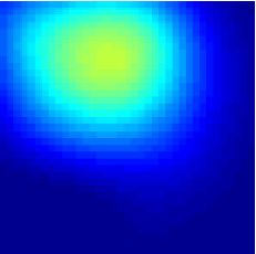
Mo, Rohrbach, and Sunar: Imaging a photodynamic therapy photosensitizer : : :
The in vivo experiments showed the fluorescence yield of HPPH 19. R. B. Schulz et al., “Comparison of noncontact and fiber-based
decreased and lifetime increased as a result of PDT. Our results fluorescence-mediated tomography,” Opt. Lett. 31(6), 769–771 (2006).
20. J. Lee and E. M. Sevick-Muraca, “Three-dimensional fluorescence
highlight the potential that TD-FDOT can provide physiological
enhanced optical tomography using referenced frequency-domain
and molecular level markers (such as fluorescence yield and life- photon migration measurements at emission and excitation wave-
time) for monitoring PDT in preclinical and clinical settings. lengths,” J. Opt. Soc. Am. A 19(4), 759–771 (2002).
21. X. Montet et al., “Tomographic fluorescence imaging of tumor vascular
volume in mice,” Radiology 242(3), 751–758 (2007).
Acknowledgments 22. A. B. Milstein et al., “Fluorescence optical diffusion tomography,” Appl.
We thank Dr. Ravindra K. Pandey for providing the drug. We Opt. 42(16), 3081–3094 (2003).
23. V. Ntziachristos et al., “Looking and listening to light: the evolution of
acknowledge Dr. Elizabeth Repasky lab for providing head and whole-body photonic imaging,” Nat. Biotechnol. 23(3), 313–320
neck mouse tumor model. We also thank Scott Galas for useful (2005).
discussions regarding image reconstructions. This research is 24. D. Kepshire et al., “Fluorescence tomography characterization for
partially supported by RPCI Startup Grant (U. Sunar) and sub-surface imaging with protoporphyrin IX,” Opt. Express 16(12),
PO1 PDT Grant [NCI CA55791 (B. W. Henderson)]. 8581–8593 (2008).
25. D. S. Kepshire et al., “Imaging of glioma tumor with endogenous fluor-
escence tomography,” J. Biomed. Opt. 14(3), 030501 (2009).
References 26. N. C. Biswal et al., “Fluorescence imaging of vascular endothelial
growth factor in tumors for mice embedded in a turbid medium,”
1. M. A. MacCormack, “Photodynamic therapy in dermatology: an update J. Biomed. Opt. 15(1), 016012 (2010).
on applications and outcomes,” Semin. Cutan. Med. Surg. 27(1), 52–62 27. J. Axelsson, J. Swartling, and S. Andersson-Engels, “In vivo photo-
(2008). sensitizer tomography inside the human prostate,” Opt. Lett. 34(3),
2. T. J. Dougherty, “An update on photodynamic therapy applications,” 232–234 (2009).
J. Clin. Laser Med. Surg. 20(1), 3–7 (2002). 28. A. Corlu et al., “Three-dimensional in vivo fluorescence diffuse optical
3. A. Juzeniene, Q. Peng, and J. Moan, “Milestones in the development of tomography of breast cancer in humans,” Opt. Express 15(11),
photodynamic therapy and fluorescence diagnosis,” Photochem. Photo- 6696–6716 (2007).
biol. Sci. 6(12), 1234–1245 (2007). 29. Y. Lin et al., “Quantitative fluorescence tomography with functional and
4. H. R. Nava et al., “Photodynamic therapy (PDT) using HPPH for the structural a priori information,” Appl. Opt. 48(7), 1328–1336 (2009).
treatment of precancerous lesions associated with barrett's esophagus,” 30. V. Venugopal et al., “Full-field time-resolved fluorescence tomography
Laser. Surg. Med. 43(7), 705–712 (2011). of small animals,” Opt. Lett. 35(19), 3189–3191 (2010).
5. R. K. Pandey et al., “Nature: a rich source for developing multifunc- 31. S. C. Davis et al., “Magnetic resonance-coupled fluorescence tomogra-
tional agents. Tumor-imaging and photodynamic therapy,” Laser. phy scanner for molecular imaging of tissue,” Rev. Sci. Instrum. 79(6),
Surg. Med. 38(5), 445–467 (2006). 064302 (2008).
6. S. K. Pandey et al., “Multimodality agents for tumor imaging (PET, 32. S. C. Davis et al., “MRI-coupled fluorescence tomography quantifies
fluorescence) and photodynamic therapy. A possible ‘see and treat’ EGFR activity in brain tumors,” Acad. Radiol. 17(3), 271–276 (2010).
approach,” J. Med. Chem. 48(20), 6286–6295 (2005).
33. W. Becker, Advanced Time-Correlated Single Photon Counting
7. U. Sunar et al., “Monitoring photobleaching and hemodynamic
Techniques, (Springer, Berlin (2005).
responses to HPPH-mediated photodynamic therapy of head and
34. J. R. Lacowicz, Principles of Fluorescence Spectroscopy (Springer,
neck cancer: a case report,” Opt. Express 18(14), 14969–14978 (2010).
Berlin 1999).
8. X. Zheng et al., “Conjugation of 2-(1'-hexyloxyethyl)-2-devinylpyro-
35. R. Cubeddu et al., “Time-resolved fluorescence imaging in biology and
pheophorbide-a (HPPH) to carbohydrates changes its subcellular distri-
medicine,” J. Phys. D 35, R61–R76 (2002).
bution and enhances photodynamic activity in vivo,” J. Med. Chem.
36. D. Hall et al., “Simple time-domain optical method for estimating the
52(14), 4306–4318 (2009).
depth and concentration of a fluorescent inclusion in a turbid medium,”
9. B. C. Wilson, M. S. Patterson, and L. Lilge, “Implicit and explicit
Opt. Lett. 29(19), 2258–2260 (2004).
dosimetry in photodynamic therapy: a new paradigm,” Laser. Med. Sci.
37. S. H. Han and D. J. Hall, “Estimating the depth and lifetime of a fluo-
12(3), 182–199 (1997).
rescent inclusion in a turbid medium using a simple time-domain optical
10. I. Georgakoudi and T. H. Foster, “Singlet oxygen- versus nonsinglet
method,” Opt. Lett. 33(9), 1035–1037 (2008).
oxygen-mediated mechanisms of sensitizer photobleaching and their
38. D. J. Hall et al., “In vivo simultaneous monitoring of two fluorophores
effects on photodynamic dosimetry,” Photochem. Photobiol. 67(6),
with lifetime contrast using a full-field time domain system,” Appl. Opt.
612–625 (1998).
48(10), D74–78 (2009).
11. Q. Peng et al., “Selective distribution of porphyrins in skin thick basal
39. A. Laidevant et al., “Analytical method for localizing a fluorescent
cell carcinoma after topical application of methyl 5-aminolevulinate,”
inclusion in a turbid medium,” Appl. Opt. 46(11), 2131–2137 (2007).
J. Photochem. Photobiol. B 62(3), 140–145 (2001).
12. S. Andersson-Engels et al., “In vivo fluorescence imaging for tissue 40. S. Lam, F. Lesage, and X. Intes, “Time domain fluorescent diffuse
diagnostics,” Phys. Med. Biol. 42(5), 815–824 (1997). optical tomography: Analytical expressions,” Opt. Express 13(7),
13. V. Ntziachristos, “Fluorescence molecular imaging,” Annu. Rev. 2263–2275 (2005).
Biomed. Eng. 8, 1–33 (2006). 41. J. Boutet et al., “Bimodal ultrasound and fluorescence approach for
14. X. D. Li et al., “Fluorescent diffuse photon density waves in homoge- prostate cancer diagnosis,” J. Biomed. Opt. 14(6), 064001 (2009).
neous and heterogeneous turbid media: analytic solutions and 42. R. E. Nothdurft et al., “In vivo fluorescence lifetime tomography,”
applications,” Appl. Opt. 35(19), 3746–3758 (1996). J. Biomed. Opt. 14(6), 024004 (2009).
15. E. E. Graves et al., “A submillimeter resolution fluorescence molecular 43. A. T. Kumar et al., “Fluorescence-lifetime-based tomography for turbid
imaging system for small animal imaging,” Med. Phys. 30(5), 901–911 media,” Opt. Lett. 30(24), 3347–3349 (2005).
(2003). 44. A. T. Kumar et al., “A time domain fluorescence tomography system for
16. S. Patwardhan et al., “Time-dependent whole-body fluorescence small animal imaging,” IEEE Trans. Med. Imag. 27(8), 1152–1163 (2008).
tomography of probe bio-distributions in mice,” Opt. Express 13(7), 45. M. A. O’Leary et al., “Fluorescence lifetime imaging in turbid media,”
2564–2577 (2005). Opt. Lett. 21(2), 158–160 (1996).
17. V. Ntziachristos and R. Weissleder, “Experimental three-dimensional 46. A. Godavarty, E. M. Sevick-Muraca, and M. J. Eppstein, “Three-
fluorescence reconstruction of diffuse media by use of a normalized dimensional fluorescence lifetime tomography,” Med. Phys. 32(4),
Born approximation,” Opt. Lett. 26(12), 893–895 (2001). 992–1000 (2005).
18. A. D. Klose and A. H. Hielscher, “Fluorescence tomography with simu- 47. F. Gao et al., “A linear, featured-data scheme for image reconstruction in
lated data based on the equation of radiative transfer,” Opt. Lett. 28(12), time-domain fluorescence molecular tomography,” Opt. Express 14(16),
1019–1021 (2003). 7109–7124 (2006).
Journal of Biomedical Optics 071306-7 July 2012 • Vol. 17(7)
Downloaded From: https://www.spiedigitallibrary.org/journals/Journal-of-Biomedical-Optics on 23 Feb 2021
Terms of Use: https://www.spiedigitallibrary.org/terms-of-use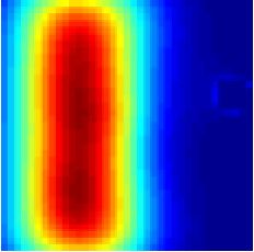
Mo, Rohrbach, and Sunar: Imaging a photodynamic therapy photosensitizer : : :

                48. J. Chen, V. Venugopal, and X. Intes, “Monte Carlo based method for             61. J. P. Connelly et al., “Time-resolved fluorescence imaging of photosen-
                    fluorescence tomographic imaging with lifetime multiplexing using                  sitiser distributions in mammalian cells using a picosecond laser line-
                    time gates,” Biomed. Opt. Express 2(4), 871–886 (2011).                            scanning microscope,” J. Photochem. Photobiol. A 142(2–3), 169–175
                49. R. Cubeddu et al., “Tumor detection in mice by measurement of fluo-                (2001).
                    rescence decay time matrices,” Opt. Lett. 20(24), 2553–2555 (1995).            62. A. T. Kumar et al., “Time resolved fluorescence tomography of turbid
                50. R. Cubeddu et al., “Use of time-gated fluorescence imaging for diagnosis           media based on lifetime contrast,” Opt. Express 14(25), 12255–12270
                    in biomedicine,” J. Photochem. Photobiol. B 12(1), 109–113 (1992).                 (2006).
                51. R. Cubeddu et al., “Time-gated fluorescence imaging for the diagnosis          63. V. Y. Soloviev et al., “Fluorescence lifetime imaging by using time-
                    of tumors in a murine model,” Photochem. Photobiol. 57(3), 480–485                 gated data acquisition,” Appl. Opt. 46(3), 7384–7391 (2007).
                    (1993).                                                                        64. A. Soubret, J. Ripoll, and V. Ntziachristos, “Accuracy of fluorescent
                52. I. Munro et al., “Toward the clinical application of time-domain fluo-             tomography in the presence of heterogeneities: study of the normalized
                    rescence lifetime imaging,” J. Biomed. Opt. 10(5), 051403 (2005).                  Born ratio,” IEEE Trans. Med. Imag. 24(10), 1377–1386 (2005).
                53. S. Bloch et al., “Whole-body fluorescence lifetime imaging of a tumor-         65. V. Ntziachristos et al., “Planar fluorescence imaging using normalized
                    targeted near-infrared molecular probe in mice,” J. Biomed. Opt. 10(5),            data,” J. Biomed. Opt. 10(6), 064007 (2005).
                    054003 (2005).                                                                 66. V. Ntziachristos and R. Weissleder, “Charge-coupled-device based scan-
                54. M. Y. Berezin et al., “Ratiometric analysis of fluorescence lifetime for           ner for tomography of fluorescent near-infrared probes in turbid media,”
                    probing binding sites in albumin with near-infrared fluorescent mole-              Med. Phys. 29(5), 803–809 (2002).
                    cular probes,” Photochem. Photobiol. 83(6), 1371–1378 (2007).                  67. M. S. Patterson, B. Chance, and B. C. Wilson, “Time resolved
                55. A. D. Scully et al., “Application of fluorescence lifetime imaging                 reflectance and transmittance for the noninvasive measurement of tissue
                    microscopy to the investigation of intracellular PDT mechanisms,”                  optical properties,” Appl. Opt. 28(12), 2331–2336 (1989).
                    Bioimaging 5(1), 9–18 (1997).                                                  68. A. C. Kak and M. Slaney, Principles of Computerized Tomographic
                56. J. A. Russell et al., “Characterization of fluorescence lifetime of Photo-         Imaging, IEEE Press, New York (1988).
                    frin and delta-aminolevulinic acid induced protoporphyrin IX in living         69. O. Mermut et al., “Frequency domain, time-resolved and spectroscopic
                    cells using single- and two-photon excitation,” IEEE J. Sel. Top. Quan-            investigations of photosensitizers encapsulated in liposomal phantoms,”
                    tum. Electron. 14(1), 158–166 (2008).                                              Proc. SPIE 6632, 66320P (2007).
                57. D. Sud et al., “Time-resolved optical imaging provides a molecular             70. M. Molls and P. Vaupel, Blood Perfusion and Microenvironment of
                    snapshot of altered metabolic function in living human cancer cell                 Human Tumors: Implications for Clinical Radiooncology, (Springer,
                    models,” Opt. Express 14(10), 4412–4426 (2006).                                    Berlin 2000).
                58. J. Siegel et al., “Studying biological tissue with fluorescence lifetime       71. B. C. Wilson and M. S. Patterson, “The physics, biophysics and
                    imaging: microscopy, endoscopy, and complex decay profiles,” Appl.                 technology of photodynamic therapy,” Phys. Med. Biol. 53(9),
                    Opt. 42(16), 2995–3004 (2003).                                                     R61–R109 (2008).
                59. D. Elson et al., “Time-domain fluorescence lifetime imaging applied to         72. T. L. Becker et al., “Monitoring blood flow responses during topical
                    biological tissue,” Photochem. Photobiol. Sci. 3(8), 795–801 (2004).               ALA-PDT,” Biomed. Opt. Express 2(1), 123–130 (2011).
                60. M. Kress et al., “Time-resolved microspectrofluorometry and fluorescence       73. S. V. Patwardhan and J. P. Culver, “Quantitative diffuse optical tomog-
                    lifetime imaging of photosensitizers using picosecond pulsed diode lasers          raphy for small animals using an ultrafast gated image intensifier,”
                    in laser scanning microscopes,” J. Biomed. Opt. 8(1), 26–32 (2003).                J. Biomed. Opt. 13(1), 011009 (2008).

                Journal of Biomedical Optics                                                071306-8                                                  July 2012   •   Vol. 17(7)

Downloaded From: https://www.spiedigitallibrary.org/journals/Journal-of-Biomedical-Optics on 23 Feb 2021
Terms of Use: https://www.spiedigitallibrary.org/terms-of-use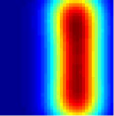
You can also read