Individual-Specific Areal-Level Parcellations Improve Functional Connectivity Prediction of Behavior
←
→
Page content transcription
If your browser does not render page correctly, please read the page content below
Cerebral Cortex, 2021;00: 1–24

                                                                              https://doi.org/10.1093/cercor/bhab101
                                                                              Original Article

                                                                                                                                                Downloaded from https://academic.oup.com/cercor/advance-article/doi/10.1093/cercor/bhab101/6263393 by Yale University user on 07 July 2021
ORIGINAL ARTICLE

Individual-Specific Areal-Level Parcellations Improve
Functional Connectivity Prediction of Behavior
Ru Kong1,2,3 , Qing Yang1,2,3 , Evan Gordon4 , Aihuiping Xue1,2,3 ,
Xiaoxuan Yan1,2,3,5 , Csaba Orban1,2,3 , Xi-Nian Zuo 6,7 ,
Nathan Spreng8,9,10 , Tian Ge11,12 , Avram Holmes13 , Simon Eickhoff14,15 and
B.T. Thomas Yeo1,2,3,5,12
1 Department of Electrical and Computer Engineering, National University of Singapore, Singapore 117583,

Singapore, 2 Centre for Sleep and Cognition (CSC) & Centre for Translational Magnetic Resonance Research
(TMR), National University of Singapore, Singapore 117549, Singapore, 3 N.1 Institute for Health and Institute
for Digital Medicine (WisDM), National University of Singapore, Singapore 117456, Singapore, 4 Department of
Radiology, Washington University School of Medicine, St. Louis, MO 63130, USA, 5 Integrative Sciences and
Engineering Programme (ISEP), National University of Singapore, Singapore 119077, Singapore, 6 State Key
Laboratory of Cognitive Neuroscience and Learning/IDG McGovern Institute for Brain Research, Beijing Normal
University, Beijing 100875, China, 7 National Basic Public Science Data Center, Chinese Academy of Sciences,
Beijing 100101, China, 8 Laboratory of Brain and Cognition, Department of Neurology and Neurosurgery, McGill
University, Montreal QC H3A 2B4, Canada, 9 Departments of Psychiatry and Psychology, Neurological Institute,
McGill University, Montreal QC H3A 2B4, Canada, 10 McConnell Brain Imaging Centre, Montreal Neurological
Institute (MNI), McGill University, Montreal QC H3A 2B4, Canada, 11 Psychiatric & Neurodevelopmental
Genetics Unit, Center for Genomic Medicine, Massachusetts General Hospital, Boston, MA 02114, USA,
12 Martinos Center for Biomedical Imaging, Massachusetts General Hospital, Charlestown, MA 02129, USA,
13 Department of Psychology, Yale University, New Haven, CT 06520, USA, 14 Medical Faculty, Institute for

Systems Neuroscience, Heinrich-Heine University Düsseldorf, Düsseldorf 40225, Germany and 15 Institute of
Neuroscience and Medicine, Brain & Behaviour (INM-7), Research Center Jülich, Jülich 52425, Germany
Address correspondence to B.T. Thomas Yeo, N.1 & WISDM, National University of Singapore, Singapore. Email: thomas.yeo@nus.edu.sg

Abstract
Resting-state functional magnetic resonance imaging (rs-fMRI) allows estimation of individual-specific cortical
parcellations. We have previously developed a multi-session hierarchical Bayesian model (MS-HBM) for estimating
high-quality individual-specific network-level parcellations. Here, we extend the model to estimate individual-specific
areal-level parcellations. While network-level parcellations comprise spatially distributed networks spanning the cortex,
the consensus is that areal-level parcels should be spatially localized, that is, should not span multiple lobes. There is
disagreement about whether areal-level parcels should be strictly contiguous or comprise multiple noncontiguous
components; therefore, we considered three areal-level MS-HBM variants spanning these range of possibilities.
Individual-specific MS-HBM parcellations estimated using 10 min of data generalized better than other approaches using
150 min of data to out-of-sample rs-fMRI and task-fMRI from the same individuals. Resting-state functional connectivity
derived from MS-HBM parcellations also achieved the best behavioral prediction performance. Among the three MS-HBM
variants, the strictly contiguous MS-HBM exhibited the best resting-state homogeneity and most uniform within-parcel
task activation. In terms of behavioral prediction, the gradient-infused MS-HBM was numerically the best, but differences

© The Author(s) 2021. Published by Oxford University Press. All rights reserved. For permissions, please e-mail: journals.permissions@oup.com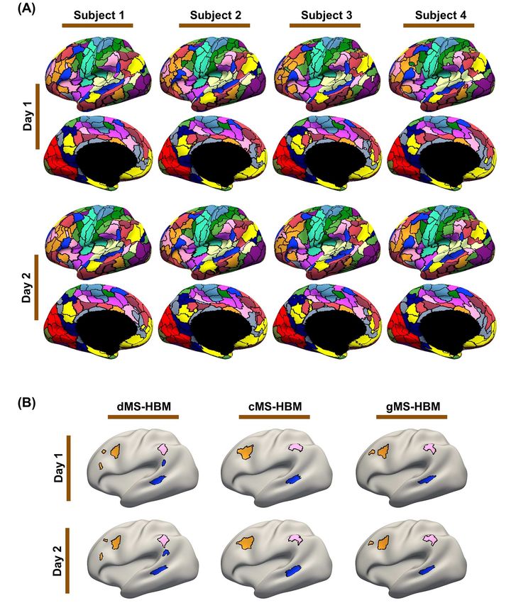
2     Cerebral Cortex, 2021, Vol. 00, No. 00

among MS-HBM variants were not statistically significant. Overall, these results suggest that areal-level MS-HBMs can
capture behaviorally meaningful individual-specific parcellation features beyond group-level parcellations. Multi-resolution
trained models and parcellations are publicly available (https://github.com/ThomasYeoLab/CBIG/tree/master/stable_proje
cts/brain_parcellation/Kong2022_ArealMSHBM).

Key words: behavioral prediction, brain parcellation, difference, individual, resting-state functional connectivity

                                                                                                                                               Downloaded from https://academic.oup.com/cercor/advance-article/doi/10.1093/cercor/bhab101/6263393 by Yale University user on 07 July 2021
Introduction                                                                 In this study, we extend the network-level MS-HBM to
                                                                         estimate individual-specific areal-level parcellations. While
The human cerebral cortex comprises hundreds of cortical areas
                                                                         network-level parcellations comprise spatially distributed
with distinct function, architectonics, connectivity, and topogra-
                                                                         networks spanning the cortex, the consensus is that areal-level
phy (Kaas 1987; Felleman and Van Essen 1991; Eickhoff, Consta-
                                                                         parcels should be spatially localized (Kaas 1987; Amunts and
ble, et al. 2018a). These areas are thought to be organized into at
                                                                         Zilles 2015), that is, an areal-level parcel should not span mul-
least 6–20 spatially distributed large-scale networks that broadly
                                                                         tiple cortical lobes. Consistent with invasive studies (Amunts
subserve distinct aspects of human cognition (Goldman-Rakic
                                                                         and Zilles 2015), most areal-level parcellation approaches
1988; Mesulam 1990; Smith et al. 2009; Bressler and Menon 2010;
                                                                         estimate spatially contiguous parcels (Shen et al. 2013; Honnorat
Uddin et al. 2019). Accurate parcellation of the cerebral cortex
                                                                         et al. 2015; Gordon et al. 2016; Chong et al. 2017). However,
into areas and networks is therefore an important problem in
                                                                         a few studies have suggested that individual-specific areal-
systems neuroscience. The advent of in vivo noninvasive brain
                                                                         level parcels can be topologically disconnected (Glasser et al.
imaging techniques, such as functional magnetic resonance
                                                                         2016; Li, Wang, et al. 2019b). For example, according to Glasser
imaging (fMRI), has enabled the delineation of cortical parcels
                                                                         et al. (2016), area 55b might comprise two disconnected, but
that approximate these cortical areas (Sereno et al. 1995; Van
                                                                         spatially close, components in some individuals. Given the lack
Essen and Glasser 2014; Eickhoff, Yeo, et al. 2018b).
                                                                         of consensus, we considered three different spatial localization
    A widely used approach for estimating network-level and
                                                                         priors. Across the three priors, the resulting parcels ranged
areal-level cortical parcellations is resting-state functional con-
                                                                         from being strictly contiguous to being spatially localized with
nectivity (RSFC). RSFC reflects the synchrony of fMRI signals
                                                                         multiple noncontiguous components.
between brain regions, while a participant is lying at rest without
                                                                             We compared MS-HBM areal-level parcellations with three
performing any explicit task, that is, resting-state fMRI (rs-fMRI;
                                                                         other approaches (Laumann et al. 2015; Schaefer et al. 2018; Li,
Biswal et al. 1995; Fox and Raichle 2007; Buckner et al. 2013).
                                                                         Wang, et al. 2019b) in terms of their generalizability to out-of-
Most RSFC studies have focused on estimating group-level par-
                                                                         sample rs-fMRI and task-fMRI from the same individuals. Fur-
cellations obtained by averaging data across many individuals
                                                                         thermore, a vast body of literature has shown that RSFC derived
(Power et al. 2011; Yeo et al. 2011; Craddock et al. 2012; Zuo et al.
                                                                         from group-level parcellations can be used to predict human
2012; Gordon et al. 2016). These group-level parcellations have
                                                                         behavior (Hampson et al. 2006; Finn et al. 2015; Rosenberg et al.
provided important insights into brain network organization but
                                                                         2016; Li, Kong, et al. 2019a). Therefore, we also investigated
fail to capture individual-specific parcellation features (Harrison
                                                                         whether RSFC derived from individual-specific MS-HBM parcel-
et al. 2015; Laumann et al. 2015; Braga and Buckner 2017; Gordon,
                                                                         lations could improve behavioral prediction compared with two
Laumann, Adeyemo, et al. 2017a). Furthermore, recent studies
                                                                         other parcellation approaches (Schaefer et al. 2018; Li, Wang,
have shown that individual-specific parcellation topography is
                                                                         et al. 2019b).
behaviorally relevant (Salehi et al. 2018; Bijsterbosch et al. 2019;
Kong et al. 2019; Mwilambwe-Tshilobo et al. 2019; Seitzman et al.
2019; Li, Wang, et al. 2019b; Cui et al. 2020), motivating significant
interest in estimating individual-specific parcellations.                Methods
    Most individual-specific parcellations only account for inter-
                                                                         Overview
subject (between-subject) variability, but not intra-subject
(within-subject) variability. However, inter-subject and intra-          We proposed the spatially constrained MS-HBM to estimate
subject RSFC variability can be markedly different across brain          individual-specific areal-level parcellations. The model distin-
regions (Mueller et al. 2013; Chen et al. 2015; Laumann et al.           guished between inter-subject and intra-subject functional con-
2015). For example, the sensory-motor cortex exhibits low inter-         nectivity variability, while incorporating spatial contiguity con-
subject variability, but high intra-subject variability (Mueller         straints. Three different contiguity constraints were considered:
et al. 2013; Laumann et al. 2015). Therefore, it is important to         distributed MS-HBM (dMS-HBM), contiguous MS-HBM (cMS-
consider both inter-subject and intra-subject variability when           HBM), and gradient-infused MS-HBM (gMS-HBM). The resulting
estimating individual-specific parcellations (Mejia et al. 2015,         MS-HBM parcels ranged from being strictly contiguous (cMS-
2018; Kong et al. 2019). We have previously proposed a multi-            HBM) to being spatially localized with multiple topologically
session hierarchical Bayesian model (MS-HBM) of individual-              disconnected components (dMS-HBM). Subsequent analyses
specific network-level parcellation that accounted for both              proceeded in four stages. First, we explored the pattern of inter-
inter-subject and intra-subject variability (Kong et al. 2019).          subject and intra-subject functional variability across the cortex.
We demonstrated that compared with several alternative                   Second, we examined the intra-subject reproducibility and inter-
approaches, individual-specific MS-HBM networks generalized              subject similarity of MS-HBM parcellations on two different
better to new resting-fMRI and task-fMRI data from the same              datasets. Third, the MS-HBM was compared with three other
individuals (Kong et al. 2019).                                          approaches using new rs-fMRI and task-fMRI data from the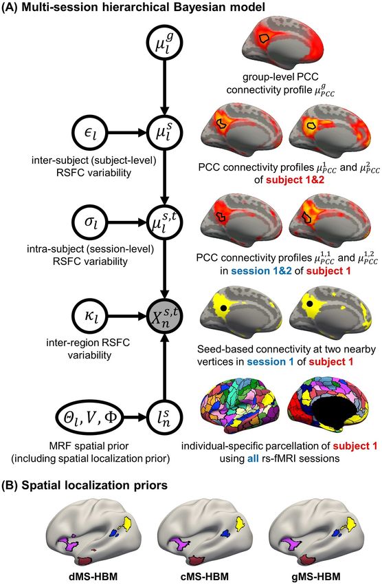
Individual-Specific Areal-Level Parcellation      Kong et al.        3

same participants. Finally, we investigated whether functional           Functional Connectivity Profiles
connectivity of individual-specific parcellations could improve
                                                                         As explained in the previous section, the preprocessed rs-fMRI
behavioral prediction.
                                                                         data from the HCP and MSC datasets have been projected onto
                                                                         fs_LR32K surface space, comprising 59 412 cortical vertices. A
Multi-session rs-fMRI Datasets                                           binarized connectivity profile of each cortical vertex was then
                                                                         computed as was done in our previous study (Kong et al. 2019).
The Human Connectome Project (HCP) S1200 release (Van Essen,
                                                                         More specifically, we considered 1483 regions of interest (ROIs)

                                                                                                                                                  Downloaded from https://academic.oup.com/cercor/advance-article/doi/10.1093/cercor/bhab101/6263393 by Yale University user on 07 July 2021
Ugurbil, et al. 2012a; Smith et al. 2013) comprised structural MRI,
                                                                         consisting of single vertices uniformly distributed across the
rs-fMRI, and task-fMRI of 1094 young adults. All imaging data
                                                                         fs_LR32K surface meshes (Kong et al. 2019). For each rs-fMRI
were collected on a custom-made Siemens 3T Skyra scanner
                                                                         run of each participant, the Pearson’s correlation between the
using a multiband sequence. Each participant went through two
                                                                         fMRI time series at each spatial location (59 412 vertices) and the
fMRI sessions on two consecutive days. Two rs-fMRI runs were
                                                                         1483 ROIs was computed. Outlier volumes were ignored when
collected in each session. Each fMRI run was acquired at 2 mm
                                                                         computing the correlations. The 59 412 × 1483 RSFC (correlation)
isotropic resolution with a time repetition (TR) of 0.72 s and
                                                                         matrices were then binarized by keeping the top 10% of the
lasted for 14 min and 33 s. The structural data consisted of one
                                                                         correlations to obtain the final functional connectivity profile
0.7 mm isotropic scan for each participant.
                                                                         (Kong et al. 2019).
    The Midnight Scanning Club (MSC) multi-session dataset
                                                                             We note that because fMRI is spatially smooth and exhibits
comprised structural MRI, rs-fMRI, and task-fMRI from 10 young
                                                                         long-range correlations, therefore considering only 1483 ROI
adults (Gordon, Laumann, Gilmore, et al. 2017b; Gratton et al.
                                                                         vertices (instead of all 59 412 vertices) would reduce compu-
2018). All imaging data were collected on a Siemens Trio 3T MRI
                                                                         tational and memory demands, without losing much informa-
scanner using a 12-channel head matrix coil. Each participant
                                                                         tion. To verify significant information has not been lost, the
was scanned for 10 sessions of rs-fMRI data. One rs-fMRI run
                                                                         following analysis was performed. For each HCP participant, a
was collected in each session. Each fMRI run was acquired at
                                                                         59 412 × 59 412 RSFC matrix was computed from the first rs-fMRI
4 mm isotropic resolution with a TR of 2.2 s and lasted for 30 min.
                                                                         run. We then correlated every pair of rows of the RSFC matrix,
The structural data were collected across two separate days and
                                                                         yielding a 59 412 × 59 412 RSFC similarity matrix for each HCP
consisted of four 0.8 mm isotropic T1-weighted images and four
                                                                         participant. An entry in this RSFC similarity matrix indicates
0.8 mm isotropic T2-weighted images.
                                                                         the similarity of the functional connectivity profiles of two
    It is worth noting some significant acquisition differences
                                                                         cortical locations. The procedure was repeated but using the
between the two datasets, including scanner type (e.g., Skyra vs.
                                                                         59 412 × 1483 RSFC matrices to compute the 59 412 × 59 412 RSFC
Trio), acquisition sequence (e.g., multiband vs. non-multiband),
                                                                         similarity matrices. Finally, for each HCP participant, we corre-
and scan time (e.g., day vs. midnight). These differences allowed
                                                                         lated the RSFC similarity matrix (generated from 1483 vertices)
us to test the robustness of our parcellation approach.
                                                                         and RSFC similarity matrix (generated from 59 412 vertices).
                                                                         The resulting correlations were high with r = 0.9832 ± 0.0041
Preprocessing                                                            (mean ± SD) across HCP participants, suggesting that very little
                                                                         information was lost by only considering 1483 vertices.
Details of the HCP preprocessing can be found elsewhere (Van
Essen, Ugurbil, et al. 2012a; Glasser et al. 2013; Smith et al. 2013;
HCP S1200 manual). Of particular importance is that the rs-              Group-Level Parcellation
fMRI data have been projected to the fs_LR32k surface space              We have previously developed a set of high-quality population-
(Van Essen, Glasser, et al. 2012b), smoothed by a Gaussian ker-          average areal-level parcellations of the cerebral cortex (Schaefer
nel with 2 mm full-width at half-maximum (FWHM), denoised                et al. 2018), which we will refer to as “Schaefer2018.” Although
with ICA-FIX (Griffanti et al. 2014; Salimi-Khorshidi et al. 2014),      the Schaefer2018 parcellations are available in different spatial
and aligned with MSMAll (Robinson et al. 2014). To eliminate             resolutions, we will mostly focus on the 400-region parcellation
global and head motion-related artifacts (Burgess et al. 2016;           in this paper (Fig. 4A), given that previous work has suggested
Siegel et al. 2017), additional nuisance regression and censoring        that there might be between 300 and 400 human cortical areas
were performed (Kong et al. 2019; Li, Kong, et al. 2019a). Nui-          (Van Essen, Glasser, et al. 2012b). The 400-region Schaefer2018
sance regressors comprised the global signal and its temporal            parcellation will be used to initialize the areal-level MS-HBM for
derivative. Runs with more than 50% censored frames were                 estimating individual-specific parcellations. The Schaefer2018
removed. Participants with all four runs remaining (N = 835) were        parcellation will also be used as a baseline in our experiments.
considered.
    In the case of the MSC dataset, we utilized the preprocessed
                                                                         Areal-Level MS-HBM
rs-fMRI data of nine subjects on fs_LR32k surface space. Pre-
processing steps included slice time correction, motion cor-             The areal-level MS-HBM (Fig. 1A) is the same as the network-
rection, field distortion correction, motion censoring, nuisance         level MS-HBM (Kong et al. 2019) except for one crucial detail,
regression, and bandpass filtering (Gordon, Laumann, Gilmore,            that is, spatial localization prior 8 (Fig. 1A). Nevertheless, for
et al. 2017b). Nuisance regressors comprised whole brain, ven-           completeness, we will briefly explain the other components of
tricular and white matter signals, as well as motion regressors          the MS-HBM, although further details can be found elsewhere
derived from Volterra expansion (Friston et al. 1996). The surface       (Kong et al. 2019).
data were smoothed by a Gaussian kernel with 6 mm FWHM.                     We denote the binarized functional connectivity profile of
                                                                                                                                 s,t
One participant (MSC08) exhibited excessive head motion and              cortical vertex n during session t of subject s as Xn . For exam-
self-reported sleep (Gordon, Laumann, Gilmore, et al. 2017b;             ple, the binarized functional connectivity profiles of a posterior
                                                                                                      1,1                                 1,1
Seitzman et al. 2019) and was thus excluded from subsequent              cingulate cortex vertex (XPCC ) and a precuneus vertex (XpCun )
analyses.                                                                from the first session of the first subject are illustrated in Fig. 1A
4 Cerebral Cortex, 2021, Vol. 00, No. 00
Downloaded from https://academic.oup.com/cercor/advance-article/doi/10.1093/cercor/bhab101/6263393 by Yale University user on 07 July 2021
s,t
Figure 1. (A) MS-HBM of individual-specific areal-level parcellations. Xn denote the RSFC profile at brain location n of subject s during rs-fMRI session t. The shaded
s,t g
circle indicates that Xn are the only observed variables. The goal is to estimate the parcel label lsn for subject s at location n given RSFC profiles from all sessions. µl is
the group-level RSFC profile of parcel l. µsl is the subject-specific RSFC profile of parcel l. A large ǫl indicates small inter-subject RSFC variability, that is, the group-level
s,t
and subject-specific RSFC profiles are very similar. µl is the subject-specific RSFC profile of parcel l during session t. A large σl indicates small intra-subject RSFC
variability, that is, the subject-level and session-level RSFC profiles are very similar. κl captures inter-region RSFC variability. A large κl indicates small inter-region
variability, that is, two locations from the same parcel exhibit very similar RSFC profiles. Finally, Θl captures inter-subject variability in the spatial distribution of
parcels, smoothness prior V encourages parcel labels to be spatially smooth, and the spatial localization prior 8 ensures each parcel is spatially localized. The spatial
localization prior 8 is the crucial difference from the original network-level MS-HBM (Kong et al. 2019). (B) Illustration of three different spatial localization priors.
Individual-specific parcellations of the same HCP participant were estimated using dMS-HBM, cMS-HBM, and gMS-HBM. Four parcels depicted in pink, red, blue, and
yellow are shown here. All four parcels estimated by dMS-HBM were spatially close together but contained two separate components. All four parcels estimated by
cMS-HBM were spatially contiguous. Three parcels (pink, red, and yellow) estimated by gMS-HBM were spatially contiguous, while the blue parcel contained two
separate components.Individual-Specific Areal-Level Parcellation Kong et al. 5
s,t
(fourth row). The shaded circle indicates that Xn are the only areas (Fischl et al. 2008). One of the most spatially variable
observed variables. Based on the observed connectivity profiles architectonic areas is hOc5, which can be located in an adja-
of “all” vertices during “all” sessions of a single subject, the goal cent sulcus away from the group-average location (Yeo et al.
is to assign a parcel label lsn for each vertex n of subject s. Even 2010a, 2010b). This variability corresponded to about 30 mm.
though a vertex’s connectivity profiles are likely to be different Therefore, similar to Glasser et al. (2016), 8 comprises a spa-
across fMRI sessions, the vertex’s parcel label was assumed to be tial localization prior constraining each individual-specific
the same across sessions. For example, the individual-specific parcel to be within 30 mm of the group-level Schaefer2018
Downloaded from https://academic.oup.com/cercor/advance-article/doi/10.1093/cercor/bhab101/6263393 by Yale University user on 07 July 2021
areal-level parcellation of the first subject using data from all parcel boundaries. We note that this prior only guarantees
available sessions is illustrated in Fig. 1A (last row). an individual-specific parcel to be spatially localized, but
The multiple layers of the areal-level MS-HBM explicitly dif- the parcel might comprise multiple distributed components
ferentiate inter-subject (between-subject) functional connectiv- (Fig. 1B left panel). We refer to this prior as dMS-HBM.
ity variability from intra-subject (within-subject) functional con- 2. cMS-HBM. In addition to the 30 mm prior from dMS-HBM,
nectivity variability (ǫl and σl in Fig. 1A). The connectivity profiles we include a spatial localization prior encouraging vertices
of two vertices belong to the same parcel will not be identical. comprising a parcel to not be too far from the parcel center,
This variability is captured by κl (Fig. 1A). Some model param- as was done in our previous study (Schaefer et al. 2018). If
eters (e.g., group-level connectivity profiles) will be estimated this spatial contiguity prior is sufficiently strong, then all
from a training set comprising multi-session rs-fMRI data from individual-specific parcels will be spatially connected (Fig. 1B
multiple subjects. A new participant (possibly from another middle panel). However, an overly strong prior will result
dataset) with single-session fMRI data could then be parcellated overly round parcels, which is not biologically plausible (Vogt
without access to the original training data. 2009). To ameliorate this issue, the estimation procedure
The Markov random field (MRF) spatial prior (Fig. 1A last starts with a very small weight on this spatial contiguity prior
row) is important because the observed functional connectivity and then progressively increases the weight to ensure spatial
profiles of individual subjects are generally very noisy. There- contiguity. Thus, we refer to this prior as cMS-HBM. We note
fore, additional priors were imposed on the parcellation. First, that requiring parcels to be spatially connected within an
the spatial smoothness prior V encouraged neighboring vertices MRF framework is nontrivial; our approach is significantly
(e.g., PCC and pCun) to be assigned to the same parcels. Second, less computationally expensive than competing approaches
the inter-subject spatial variability prior Θl,n denote the probabil- (Nowozin and Lampert 2010; Honnorat et al. 2015).
ity of parcel l occurring at a particular spatial location n. The two 3. gMS-HBM. A well-known areal-level parcellation approach
priors (V and Θl,n ) are also present in the network-level MS-HBM is the local gradient approach, which detects local abrupt
(Kong et al. 2019). changes (i.e., gradients) in RSFC across the cortex (Cohen
However, an additional spatial prior is necessary because of et al. 2008). Our previous study (Schaefer et al. 2018) has
well-documented long-range connections spanning the cortex. suggested the utility of combining local gradient (Cohen
Therefore, with the original MRF prior (Kong et al. 2019), brain et al. 2008; Gordon et al. 2016) and global clustering (Yeo
locations with similar functional connectivity profiles could be et al. 2011) approaches for estimating areal-level parcella-
grouped together regardless of spatial proximity. In the case tions. Therefore, we complemented the spatial contiguity
of network-level MS-HBM, this is appropriate because large- prior in cMS-HBM with a prior based on local gradients in
scale networks are spatially distributed, for example, the default RSFC, which encouraged adjacent brain locations with gentle
network spans frontal, parietal, temporal, and cingulate cortices. changes in functional connectivity to be grouped into the
In the case of areal-level parcellations, there is the expectation same parcel. In practice, we found that the gradient-infused
that a single parcel should not span large spatial distances prior, together with a very weak spatial contiguity prior,
(Glasser et al. 2016; Gordon et al. 2016; Schaefer et al. 2018). dramatically increased the number of spatially contiguous
Therefore, the areal-level MS-HBM incorporates an additional parcels (Fig. 1B right panel). Furthermore, the parcels are also
prior 8 constraining parcels to be spatially localized (Fig. 1A last less round than cMS-HBM, which is in our opinion more
row). biologically plausible. We refer to this prior as gMS-HBM.
As mentioned in the Introduction, even though there is con-
A more detailed mathematical explanation of the model can
sensus that individual-specific areal-level parcels should be
be found in Supplementary Methods S1. Given a dataset of sub-
spatially localized, there are differing opinions about whether
jects with multi-session rs-fMRI data, a variational Bayes expec-
they should be spatially contiguous. Some studies have enforced
tation–maximization (VBEM) algorithm can be used to estimate
spatially contiguous cortical parcels (Laumann et al. 2015; Gor-
the following model parameters (Kong et al. 2019): group-level
don et al. 2016; Chong et al. 2017) consistent with invasive g
parcel connectivity profiles µl , the inter-subject functional con-
studies (Amunts and Zilles 2015). Other studies have estimated
nectivity variability ǫl , the intra-subject functional connectivity
parcels that might comprise multiple spatially close compo-
variability σl , the spatial smoothness prior V, and the inter-
nents (Glasser et al. 2016; Li, Wang, et al. 2019b). For example,
subject spatial variability prior Θl . The individual-specific areal-
Glasser and colleagues suggested that area 55b might be split
level parcellation of a new participant could then be generated
into two disconnected components in close spatial proximity.
using these estimated group-level priors without access to the
Given the lack of consensus, we consider three possible spatial
original training data. Furthermore, although the model requires
localization priors (i.e., 8in Fig. 1A):
multi-session fMRI data for parameter estimation, it can be
1. dMS-HBM. Previous studies have suggested that after reg- applied to a single-session fMRI data from a new participant
istering cortical folding patterns, interindividual variability (Kong et al. 2019). Details of the VBEM algorithm can be found
in architectonic locations are different across architectonic in Supplementary Methods S2.6 Cerebral Cortex, 2021, Vol. 00, No. 00
Characterizing Inter-subject and Intra-Subject Finally, the dice coefficients were averaged across all parcels
Functional Connectivity Variability to provide an overall measure of inter-subject parcellation
similarity.
Previous studies have shown that sensory-motor regions exhibit
To evaluate whether the parameters of MS-HBM algorithms
lower inter-subject, but higher intra-subject functional connec-
from one dataset could be generalized to another dataset with
tivity variability than association regions (Mueller et al. 2013;
different acquisition protocols and preprocessing pipelines, we
Laumann et al. 2015; Kong et al. 2019). Therefore, we first eval-
used the HCP model parameters to estimate individual-specific
uate whether estimates of areal-level inter-subject and intra-
Downloaded from https://academic.oup.com/cercor/advance-article/doi/10.1093/cercor/bhab101/6263393 by Yale University user on 07 July 2021
parcellations in the MSC dataset. More specifically, the MS-HBM
subject variability were consistent with previous work (Fig. 2A).
parcellations were independently estimated using the first five
The HCP dataset was divided into training (N = 40), validation
sessions and the last five sessions for each MSC participant
(N = 40), and test (N = 755) sets. Each HCP participant underwent
(Fig. 2B).
two fMRI sessions on two consecutive days. Within each session,
there were two rs-fMRI runs. All four runs were utilized.
The parameters of three MS-HBM variants (dMS-HBM, cMS- Geometric Properties of MS-HBM Parcellations
HBM, and gMS-HBM) were estimated. More specifically, the
g The three MS-HBM variants impose different spatial priors on
group-level parcel connectivity profiles µl , the inter-subject
areal-level parcellations. To characterize the geometric proper-
RSFC variability ǫl , the intra-subject RSFC variability σl , and
ties of the MS-HBM parcels (Fig. 2C), the three trained models
inter-subject spatial variability prior Θl were estimated using
(dMS-HBM, cMS-HBM, and gMS-HBM) were applied to the HCP
the HCP training set (Fig. 2A). We tuned the “free” parameters
test set using all four rs-fMRI runs. We then computed two met-
(associated with the spatial smoothness prior V and spatial
rics to characterize the geometry of the parcellations. First, for
localization prior 8) using the HCP validation set (Fig. 2A). The
each parcellation, the number of spatially disjoint components
Schaefer2018 400-region group-level parcellation (Fig. 4A) was
was computed for each parcel and averaged across all parcels.
used to initialize the optimization procedure. The final trained
Second, for each parcellation, a roundness metric was computed
MS-HBMs (Fig. 2A) were used in all subsequent analyses.
for each parcel and averaged across all parcels. Here, the round-
#parcel boundary vertices
ness of a parcel is defined as 1 − #vertices contained in the parcel ; a
Intra-Subject Reproducibility and Inter-subject larger value indicates that a parcel is rounder.
Similarity of MS-HBM Parcellations
Within-subject reliability is important for clinical applications Comparison with Alternative Approaches
(Shehzad et al. 2009; Birn et al. 2013; Zuo and Xing 2014; Zuo et al.
2019). Having verified that the spatial patterns of inter-subject Here, we compared the three MS-HBM approaches (dMS-HBM,
and intra-subject functional connectivity variability were con- cMS-HBM, and gMS-HBM) with three alternative approaches.
sistent with previous work, we further characterized the intra- The first approach was to apply the Schaefer2018 400-region
subject reproducibility and inter-subject similarity of individual- group-level parcellation to individual subjects. The second
specific MS-HBM parcellations (Fig. 2B). The three trained mod- approach is the well-known gradient-based boundary mapping
els (dMS-HBM, cMS-HBM, and gMS-HBM) were applied to the algorithm that has been widely utilized to estimate individual-
HCP test set. Individual-specific MS-HBM parcellations were specific areal-level parcellation (Laumann et al. 2015; Gordon,
independently estimated using the first two runs (day 1) and the Laumann, Gilmore, et al. 2017b). We will refer to this second
last two runs (day 2). approach as “Laumann2015” (https://sites.wustl.edu/peterse
To evaluate the reproducibility of individual-specific parcel- nschlaggarlab/resources). The third approach is the recent
lations, the Dice coefficient was computed for each parcel from individual-specific areal-level parcellation algorithm of Li,
the two parcellations of each participant: Wang, et al. (2019b) (http://nmr.mgh.harvard.edu/bid/DownLoa
d.html), which we will refer to as “Li2019.”
2 × #vertices that overlap between parcels l1s and l2s Evaluating the quality of individual-specific resting-state
Dice l1s , l2s =
#vertices in parcel l1s + #vertices in parcel l2s parcellations is difficult because of a lack of ground truth.
Here, we considered two common evaluation metrics (Gordon
where l1s and l2s are parcel l from the two parcellations of subject et al. 2016; Chong et al. 2017; Schaefer et al. 2018; Kong
s. The Dice coefficient is widely used for comparing parcellation et al. 2019): resting-state connectional homogeneity and
or segmentation overlap (Destrieux et al. 2010; Sabuncu et al. task functional inhomogeneity (i.e., uniform task activa-
2010; Birn et al. 2013; Blumensath et al. 2013; Arslan et al. 2015; tion; see below). These metrics encode the principle that if
Honnorat et al. 2015; Salehi et al. 2018). The Dice coefficient is an individual-specific parcellation captured the areal-level
equal to 1 if there is perfect overlap between parcels and zero organization of the individual’s cerebral cortex, then each
if there is no overlap between parcels. The Dice coefficients parcel should have homogeneous connectivity and function.
were averaged across all participants to provide insights into Furthermore, we also compared the relative utility of the
regional variation in intra-subject parcel similarity. Finally, the different parcellation approaches for RSFC-based behavioral
Dice coefficients were averaged across all parcels to provide an prediction.
overall measure of intra-subject parcellation reproducibility.
To evaluate inter-subject parcellation similarity, for each pair
Resting-State Connectional Homogeneity
of participants, the Dice coefficient was computed for each
parcel. Since there were two parcellations for each participant, Resting-state connectional homogeneity was defined as the
there were a total of four Dice coefficients for each parcel, averaged Pearson’s correlations between rs-fMRI time courses
which were then averaged. Furthermore, the Dice coefficients of all pairs of vertices within each parcel, adjusted for parcel
were averaged across all pairs of participants to provide size and summed across parcels (Schaefer et al. 2018; Kong
insights into regional variation in inter-subject parcel similarity. et al. 2019). Higher resting-state homogeneity means thatIndividual-Specific Areal-Level Parcellation Kong et al. 7
Downloaded from https://academic.oup.com/cercor/advance-article/doi/10.1093/cercor/bhab101/6263393 by Yale University user on 07 July 2021
Figure 2. Flowcharts of analyses characterizing MS-HBMs. (A) Training MS-HBMs with HCP training and validation sets, as well as characterizing inter-subject and
intra-subject RSFC variability. (B) Exploring intra-subject reproducibility and inter-subject similarity of MS-HBM parcellations using HCP test set and MSC dataset. (C)
Characterizing geometric properties of MS-HBM parcellations using HCP test set. Shaded boxes (HCP test set and MSC dataset) were solely used for evaluation and not
used at all for training or tuning the MS-HBM models.
vertices within the same parcel share more similar time courses. For each participant from the HCP test set (N = 755), we
Therefore, higher resting-state homogeneity indicates better used one run to infer the individual-specific parcellation and
parcellation quality. computed resting-state homogeneity with the remaining three8 Cerebral Cortex, 2021, Vol. 00, No. 00
runs. For the MSC dataset (N = 9), we used one session to infer a post hoc processing of MS-HBM parcellations to match the
the individual-specific parcellation and computed resting-state number of parcels and unlabeled vertices of Laumann2015 par-
homogeneity with the remaining nine sessions (Fig. 3A). cellations (Supplementary Methods S3).
Because MSC participants have large amount of rs-fMRI data In addition, the Laumann2015 approach yielded different
(300 min), we also parcellated each MSC participant using dif- numbers of parcels within an individual with different lengths of
ferent length of rs-fMRI data (10–150 min) and evaluated the rs-fMRI data. Therefore, Laumann2015 was also excluded from
resting-state homogeneity with the remaining five sessions. the analysis of out-of-sample resting-state homogeneity with
Downloaded from https://academic.oup.com/cercor/advance-article/doi/10.1093/cercor/bhab101/6263393 by Yale University user on 07 July 2021
This allowed us to estimate how much the algorithms would different lengths of rs-fMRI data (Fig. 3B).
improve with more data (Fig. 3B).
When comparing resting-state homogeneity between parcel-
lations, the effect size (Cohen’s d) of differences and a two-sided
RSFC-Based Behavioral Prediction
paired-sample t-test (dof = 754 for HCP, dof = 8 for MSC) were
computed. Most studies utilized a group-level parcellation to derive RSFC
for behavioral prediction (Dosenbach et al. 2010; Finn et al.
2015; Dubois et al. 2018; Weis et al. 2020; Li, Kong, et al. 2019a).
Task Functional Inhomogeneity
Here, we investigated if RSFC derived from individual-specific
Task functional inhomogeneity was defined as the standard parcellations can improve behavioral prediction performance.
deviation (SD) of (activation) z-values within each parcel for As before (He et al. 2020; Kong et al. 2019; Li, Kong, et al. 2019a),
each task contrast, adjusted for parcel size and summed across we considered 58 behavioral phenotypes measuring cognition,
parcels (Gordon, Laumann, Gilmore, et al. 2017b; Schaefer et al. personality, and emotion from the HCP dataset. Three partici-
2018). Lower task inhomogeneity means that activation within pants were excluded from further analyses because they did not
each parcel is more uniform. Therefore, lower task inhomogene- have all behavioral phenotypes, resulting in a final set of 752 test
ity indicates better parcellation quality. The HCP task-fMRI data participants.
consisted of seven task domains: social cognition, motor, gam- The different parcellation approaches were applied to each
bling, working memory, language processing, emotional pro- HCP test participant using all four rs-fMRI runs (Fig. 3D). The Lau-
cessing, and relational processing (Barch et al. 2013). The MSC mann2015 approach yielded parcellations with different num-
task-fMRI data consisted of three task domains: motor, mixed, bers of parcels across participants, so there was a lack of inter-
and memory (Gordon, Laumann, Gilmore, et al. 2017b). Each subject parcel correspondence. Therefore, we were unable to
task domain contained multiple task contrasts. All available task perform behavioral prediction with the Laumann2015 approach,
contrasts were utilized. so Laumann2015 was excluded from this analysis.
For each participant from the HCP test set (N = 755) and Given 400-region parcellations from different approaches
MSC dataset (N = 9), all rs-fMRI sessions were used to infer the (Schaefer2018; Li2019; dMS-HBM, cMS-HBM, gMS-HBM), func-
individual-specific parcellation (Fig. 3C). The individual-specific tional connectivity was computed by correlating averaged
parcellation was then used to evaluate task inhomogeneity time courses of each pair of parcels, resulting in a 400 × 400
for each task contrast and then averaged across all available RSFC matrix for each HCP test participant (Fig. 3D). Consistent
contrasts within a task domain, resulting in a single task with our previous work (He et al. 2020; Kong et al. 2019; Li,
inhomogeneity measure per task domain. When comparing Wang, et al. 2019b), kernel regression was utilized to predict
between parcellations, we averaged the task inhomogeneity each behavioral measure in individual participants. Suppose
metric across all contrasts within a task domain before the y is the behavioral measure (e.g., fluid intelligence) and FC
effect size (Cohen’s d) of differences and a two-sided paired- is the functional connectivity matrix of a test participant.
sample t-test (dof = 754 for HCP, dof = 8 for MSC) were computed In addition, suppose yi is the behavioral measure (e.g., fluid
for each domain. intelligence) and FCi is the individual-specific functional
connectivity matrix of the ith training participant. Then
kernel regression would predict the behavior of the test
Methodological Considerations
participant as the weighted average of the behaviors of the
It is important to note that a parcellation with more parcels training participants: y ≈ i∈training set Similarity(FCi , FC)yi . Here,
P
tends to have smaller parcel size, leading to higher resting- Similarity(FCi , FC) is the Pearson’s correlation between the
state homogeneity and lower task inhomogeneity. For example, functional connectivity matrices of the ith training participant
if a parcel comprised two vertices, then the parcel would and the test participant. Because the functional connectivity
be highly homogeneous. In our experiments, the MS-HBM matrices were symmetric, only the lower triangular portions of
algorithms and Li2019 were initialized with the 400-region the matrices were considered when computing the correlation.
Schaefer2018 group-level parcellation, resulting in the same Therefore, kernel regression encodes the intuitive idea that
number of parcels as Schaefer2018, that is, 400 parcels. This participants with more similar RSFC patterns exhibited similar
allowed for a fair comparison among MS-HBMs, Li2019, and behavioral measures.
Schaefer2018. In practice, an l2 -regularization term (i.e., kernel ridge regres-
However, parcellations estimated by Laumann2015 had a sion) was included to reduce overfitting (Supplementary Meth-
variable number of parcels across participants. Furthermore, ods S4; Murphy 2012). We performed 20-fold cross-validation
Laumann2015 parcellations also had a significant number of for each behavioral phenotype. Family structure within the HCP
vertices between parcels that were not assigned to any parcel, dataset was taken into account by ensuring participants from
which has the effect of artificially increasing resting homogene- the same family (i.e., with either the same mother ID or father
ity and decreasing task inhomogeneity. Therefore, when com- ID) were kept within the same fold and not split across folds.
paring MS-HBM with Laumann2015 using resting-state homo- For each test fold, an inner-loop 20-fold cross-validation was
geneity (Fig. 3A) and task inhomogeneity (Fig. 3C), we performed repeatedly applied to the remaining 19 folds with differentIndividual-Specific Areal-Level Parcellation Kong et al. 9
Downloaded from https://academic.oup.com/cercor/advance-article/doi/10.1093/cercor/bhab101/6263393 by Yale University user on 07 July 2021
Figure 3. Flowcharts of comparisons with other algorithms. (A) Comparing out-of-sample resting-state homogeneity across different parcellation approaches applied
to a single rs-fMRI session. (B) Comparing out-of-sample resting-state homogeneity across different parcellation approaches applied to different lengths of rs-fMRI
data. (C) Comparing task inhomogeneity across different approaches. (D) Comparing RSFC-based behavioral prediction accuracies across different approaches. Across
all analyses, MS-HBM parcellations were estimated using the trained models from Figure 2A. We remind the reader that the trained MS-HBMs were estimated using
the HCP training and validation sets (Fig. 2A), which did not overlap with the HCP test set utilized in the current set of analyses. In the case of analyses (A) and (B),
only a portion of rs-fMRI data was used to estimate the parcellations. The remaining rs-fMRI data were used to compute out-of-sample resting-state homogeneity. For
analyses (C) and (D), all available rs-fMRI data were used to estimate the parcellations. Finally, we note that the local gradient approach (Laumann2015) does not yield
a fixed number of parcels. Thus, the number of parcels is variable within an individual with different lengths of rs-fMRI data, so Laumann2015 was not considered for
analysis B. Similarly, the number of parcels is different across participants, so the sizes of the RSFC matrices are different across participants. Therefore, Laumann2015
was also not utilized for analysis D.10 Cerebral Cortex, 2021, Vol. 00, No. 00
regularization parameters. The optimal regularization parame- differences. After confirming previous literature (Mueller et al.
ter from the inner-loop cross-validation was then used to pre- 2013; Laumann et al. 2015; Kong et al. 2019) that inter-subject and
dict the behavioral phenotype in the test fold. Accuracy was intra-subject RSFC variabilities were different across the cortex,
measured by correlating the predicted and actual behavioral we then established that the MS-HBM algorithms produced
measure across all participants within the test fold (Finn et al. individual-specific areal-level parcellations with better quality
2015; Kong et al. 2019; Li, Wang, et al. 2019b). By repeating the than other approaches. Finally, we investigated whether RSFC
procedure for each test fold, each behavior yielded 20 correla- derived from MS-HBM parcellations could be used to improve
Downloaded from https://academic.oup.com/cercor/advance-article/doi/10.1093/cercor/bhab101/6263393 by Yale University user on 07 July 2021
tion accuracies, which were then averaged across the 20 folds. behavioral prediction.
Because a single 20-fold cross-validation might be sensitive
to the particular split of the data into folds (Varoquaux et al.
Sensory-Motor Cortex Exhibits Lower Inter-Subject but
2017), the above 20-fold cross-validation was repeated 100 times.
Higher Intra-Subject Functional Connectivity Variability
The mean accuracy and SD across the 100 cross-validations
will be reported. When comparing between parcellations, a cor-
Than Association Cortex
rected resampled t-test for repeated k-fold cross-validation was The parameters of gMS-HBM, dMS-HBM and cMS-HBM were
performed (Bouckaert and Frank 2004). We also repeated the estimated using the HCP training set. Supplementary Figure S1
analyses using coefficient of determination (COD) as a metric shows the inter-subject RSFC variability (ǫl ) and intra-subject
of prediction performance. RSFC variability (σl ) overlaid on corresponding Schaefer2018
As certain behavioral measures are known to correlate with group-level parcels. The pattern of inter-subject and intra-
motion (Siegel et al. 2017), we regressed out age, sex, framewise subject RSFC variability was consistent with previous work
displacement, DVARS, body mass index, and total brain volume (Mueller et al. 2013; Laumann et al. 2015; Kong et al. 2019). More
from the behavioral data before kernel ridge regression. To pre- specifically, sensory-motor parcels exhibited lower inter-subject
vent any information leak from the training data to test data, RSFC variability than association cortical parcels. On the other
the nuisance regression coefficients were estimated from the hand, association cortical parcels exhibited lower intra-subject
training folds and applied to the test fold. RSFC variability than sensory-motor parcels.
Code and Data Availability Individual-Specific MS-HBM Parcellations Exhibit High
Intra-Subject Reproducibility and Low Inter-Subject
Code for this work is freely available at the GitHub repository
Similarity
maintained by the Computational Brain Imaging Group (https://
github.com/ThomasYeoLab/CBIG). The Schaefer2018 group- To assess intra-subject reproducibility and inter-subject similar-
level parcellation and code are available here (https://github. ity, the three MS-HBM variants were tuned on the HCP train-
com/ThomasYeoLab/CBIG/tree/master/stable_projects/brain_ ing and validation sets and then applied to the HCP test set.
parcellation/Schaefer2018_LocalGlobal), while the areal-level Individual-specific parcellations were generated by using rs-
MS-HBM parcellation code is available here (https://github.com/ fMRI data from day 1 (first 2 runs) and day 2 (last 2 runs)
ThomasYeoLab/CBIG/tree/master/stable_projects/brain_parce separately for each participant. All 400 parcels were present in
llation/Kong2022_ArealMSHBM). We have also provided trained 99% of the participants.
MS-HBM parameters at different spatial resolutions, ranging Figure 4 shows the inter-subject and intra-subject spatial
from 100 to 1000 parcels. similarity (Dice coefficient) of parcels from the three MS-HBM
We note that the computational bottleneck for gMS-HBM is variants in the HCP test set. Intra-Subject reproducibility was
the computation of the local gradients (Laumann et al. 2015). greater than inter-subject similarity across all parcels. Con-
We implemented a faster and less memory-intensive version of sistent with our previous work on individual-specific cortical
the local gradient computation by subsampling the functional networks (Kong et al. 2019), sensory-motor parcels were more
connectivity matrices (Supplementary Methods S1.3). Comput- spatially similar across participants than association cortical
ing the gradient map of a single HCP run requires 15 min and parcels. Sensory-motor parcels also exhibited greater within-
3 GB of RAM, compared with 4 h and 40 GB of RAM in the subject reproducibility than association cortical parcels.
original version. The resulting gradient maps were highly sim- Overall, gMS-HBM, dMS-HBM, and cMS-HBM achieved intra-
ilar to the original gradient maps (r = 0.97). The faster gradient subject reproducibility of 81.0%, 80.4%, and 76.1%, respectively,
code can be found here (https://github.com/ThomasYeoLab/CBI and inter-subject similarity of 68.2%, 68.1%, and 63.9%, respec-
G/tree/master/utilities/matlab/speedup_gradients). tively. We note that these metrics cannot be easily used to
The individual-specific parcellations for the HCP and MSC, judge the quality of the parcellations. For example, gMS-HBM
together with the associated RSFC matrices, are available here has higher intra-subject reproducibility and higher inter-subject
(https://balsa.wustl.edu/study/show/Pr8jD and https://github. similarity than cMS-HBM, so we cannot simply conclude that
com/ThomasYeoLab/CBIG/tree/master/stable_projects/brain_ one is better than the other.
parcellation/Kong2022_ArealMSHBM). Figure 5A and Supplementary Figure S2 show the gMS-HBM
parcellations of four representative HCP participants. Supple-
mentary Figures S3 and S4 show the dMS-HBM and cMS-HBM
Results parcellations of the same HCP participants. Consistent with pre-
vious studies of individual-specific parcellations (Glasser et al.
Overview
2016; Chong et al. 2017; Gordon, Laumann, Gilmore, et al. 2017b;
Three variations of the MS-HBM with different contiguity Salehi et al. 2018; Seitzman et al. 2019; Li, Wang, et al. 2019b), par-
constraints (Fig. 1) were applied to two multi-session rs-fMRI cel shape, size, location, and topology were variable across par-
datasets to ensure that the approaches were generalizable ticipants. Parcellations were highly similar within each partic-
across datasets with significant acquisition and processing ipant with individual-specific parcel features highly preservedIndividual-Specific Areal-Level Parcellation Kong et al. 11
Downloaded from https://academic.oup.com/cercor/advance-article/doi/10.1093/cercor/bhab101/6263393 by Yale University user on 07 July 2021
Figure 4. Individual-specific MS-HBM parcellations show high within-subject reproducibility and low across-subject similarity in the HCP test set. (A) The 400-
region Schaefer2018 group-level parcellation. (B) Inter-Subject spatial similarity for different parcels. (C) Intra-Subject reproducibility for different parcels. Yellow color
indicates higher overlap. Red color indicates lower overlap. Individual-specific MS-HBM parcellations were generated by using day 1 (first two runs) and day 2 (last two
runs) separately for each participant. Sensory-motor parcels exhibited higher intra-subject reproducibility and inter-subject similarity than association parcels.
across sessions (Fig. 5B). Similar results were obtained with dMS- and 67.8%, respectively, and inter-subject similarity of 50.6%,
HBM and cMS-HBM (Fig. 5B). 47.1%, and 42.9%, respectively.
The trained MS-HBM from the HCP dataset was also applied
to the MSC dataset. The MS-HBM parcellations of four repre-
Geometric Properties of MS-HBM Parcellations
sentative MSC participants are shown in Supplementary Figures
S5–S7. Similar to the HCP dataset, the parcellations also captured In the HCP test set, the average number of spatially disconnected
unique features that were replicable across the first five sessions components per parcel was 1.95 ± 0.29 (mean ± SD), 1 ± 0, and
and the last five sessions. Overall, gMS-HBM, dMS-HBM, and 1.06 ± 0.07 for dMS-HBM, cMS-HBM, and gMS-HBM, respectively.
cMS-HBM achieved intra-subject reproducibility of 75.5%, 73.9%, In the case of dMS-HBM, the maximum number of spatially12 Cerebral Cortex, 2021, Vol. 00, No. 00
Downloaded from https://academic.oup.com/cercor/advance-article/doi/10.1093/cercor/bhab101/6263393 by Yale University user on 07 July 2021
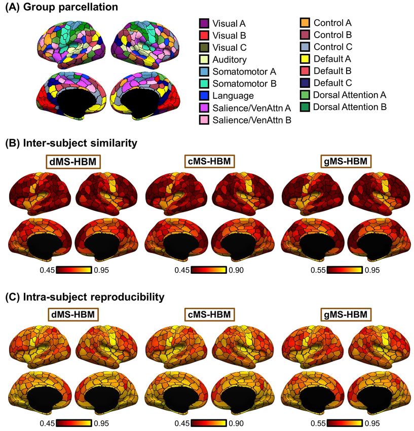
Figure 5. MS-HBM parcellations exhibit individual-specific features that are replicable across sessions. (A) The 400-region individual-specific gMS-HBM parcellations
were estimated using rs-fMRI data from day 1 and day 2 separately for each HCP test participant. Right hemisphere parcellations are shown in Supplementary Figure S2.
See Supplementary Figures S3 and S4 for dMS-HBM and cMS-HBM. (B) Replicable individual-specific parcellation features in a single HCP test participant for dMS-HBM,
cMS-HBM, and gMS-HBM.
disconnected components (across all participants and parcels) S8). On the other hand, the average roundness of the parcel-
was 11 (Supplementary Fig. S8). In the case of gMS-HBM, lations was 0.56 ± 0.02 (mean ± SD), 0.60 ± 0.01, and 0.58 ± 0.02
the maximum number of spatially disconnected components for dMS-HBM, cMS-HBM, and gMS-HBM, respectively. Overall,
(across all participants and parcels) was 3 (Supplementary Fig. gMS-HBM parcels have much fewer spatially disconnectedIndividual-Specific Areal-Level Parcellation Kong et al. 13
components than dMS-HBM, while achieving intermediate of rs-fMRI data, suggesting that MS-HBM models were able to
roundness between dMS-HBM and cMS-HBM. improve with more rs-fMRI data.
Furthermore, using just 10 min of rs-fMRI data, the MS-
HBM algorithms achieved better homogeneity than Lau-
Individual-Specific MS-HBM Parcels Exhibit Higher
mann2015 and Li2019 using 150 min of rs-fMRI data (Fig. 7B
Resting-State Homogeneity Than Other Approaches and Supplementary Fig. S10). More specifically, compared with
Individual-specific areal-level parcellations were estimated Laumann2015 using 150 min of rs-fMRI data, dMS-HBM, cMS-
Downloaded from https://academic.oup.com/cercor/advance-article/doi/10.1093/cercor/bhab101/6263393 by Yale University user on 07 July 2021
using a single rs-fMRI session for each HCP test participant HBM, and gMS-HBM using 10 min of rs-fMRI data achieved
and each MSC participant. Resting-state homogeneity was an improvement of 2.6% (Cohen’s d = 2.7, P = 3.6e−5), 6.2%
evaluated using leave-out sessions in the HCP (Fig. 6A,B) and (Cohen’s d = 5.5, P = 1.9e−7), and 5.6% (Cohen’s d = 6.1, P = 2.3e−7),
MSC (Fig. 6C,D and Supplementary Fig. S9) datasets. We note that respectively. Compared with Li2019 using 150 min of rs-fMRI
comparisons with Laumann2015 are shown on separate plots data, dMS-HBM, cMS-HBM, and gMS-HBM using 10 min of rs-
(Fig. 6B,D) because Laumann2015 yielded different number of fMRI data achieved an improvement of 0.4% (Cohen’s d = 0.4,
parcels across participants. Therefore, we matched the number not significant), 2.4% (Cohen’s d = 1.9, P = 4.3e−4), and 1.5%
of MS-HBM parcels to Laumann2015 for each participant for fair (Cohen’s d = 1.7, P = 1.0e−3), respectively. All reported P values
comparison (see Methods). were significant after correcting for multiple comparisons with
Across both HCP and MSC datasets, the MS-HBM algorithms FDR q < 0.05.
achieved better homogeneity than the group-level parcellation
(Schaefer2018) and two individual-specific areal-level parcel-
lation approaches (Laumann2015 and Li2019). Compared with Individual-Specific MS-HBM Parcels Exhibit Lower
Schaefer2019, the three MS-HBM variants achieved an improve- Task Inhomogeneity Than Other Approaches
ment ranging from 3.4% to 7.5% across the two datasets (average
Individual-specific parcellations were estimated using all rs-
improvement = 5.2%, average Cohen’s d = 3.8, largest P = 1.9e−6).
fMRI sessions from the HCP test set and MSC dataset. Task
Compared with Li2019, the three MS-HBM variants achieved
inhomogeneity was evaluated using task fMRI. Figure 8 and
an improvement ranging from 2.2% to 4.9% across the two
Supplementary Figure S11 show the task inhomogeneity of
datasets (average improvement = 3.4%, average Cohen’s d = 3.9,
all approaches for all task domains in the MSC and HCP
largest P = 5.5e−6). Compared with Laumann2015, the three MS-
datasets, respectively. Compared with Schaefer2019, the three
HBM variants achieved an improvement ranging from 6.3% to
MS-HBM variants achieved an improvement ranging from
7.8% across the two datasets (average improvement = 6.7%, aver-
0.9% to 5.9% across all task domains and datasets (average
age Cohen’s d = 7.5, largest P = 1.2e−9). All reported P values were
improvement = 3.2%, average Cohen’s d = 2.4, largest P = 2.0e−3).
significant after correcting for multiple comparisons with false
Compared with Li2019, the three MS-HBM variants achieved an
discovery rate (FDR) q < 0.05.
improvement ranging from 0.8% to 5.0% across all task domains
Among the three MS-HBM variants, cMS-HBM achieved
and datasets (average improvement = 2.7%, average Cohen’s
the highest homogeneity, while dMS-HBM was the least
d = 2.2, largest P = 1.8e−3). Compared with Laumann2015, the
homogeneous. In the HCP dataset, cMS-HBM achieved an
three MS-HBM variants achieved an improvement ranging from
improvement of 0.19% (Cohen’s d = 0.5, P = 3.5e−38) over gMS-
1.9% to 28.1% across all task domains and datasets (average
HBM, and gMS-HBM achieved an improvement of 0.76% (Cohen’s
improvement = 6.7%, average Cohen’s d = 2.3, largest P = 0.017).
d = 2.5, P = 3.5e−38) over dMS-HBM. In the MSC dataset, cMS-HBM
All reported P values were significant after correcting for
achieved an improvement of 1.1% (Cohen’s d = 3.5, P = 6.3e−6)
multiple comparisons with FDR q < 0.05. In the case of MSC,
over gMS-HBM, and gMS-HBM achieved an improvement of 0.7%
these improvements were observed in almost every single
(Cohen’s d = 2.6, P = 6.1e−5) over dMS-HBM. All reported P values
participant across all tasks (Fig. 8).
were significant after correcting for multiple comparisons with
Among the three MS-HBM variants, cMS-HBM achieved
FDR q < 0.05.
the best task inhomogeneity, while dMS-HBM achieved the
Individual-specific parcellations were estimated with
worst task inhomogeneity. Compared with gMS-HBM, cMS-HBM
increasing length of rs-fMRI data in the MSC dataset. Resting-
achieved an improvement ranging from 0.03% to 0.92% across
state homogeneity was evaluated using leave-out sessions
all task domains and datasets (average improvement = 0.3%,
(Fig. 7A and Supplementary Fig. S10). We note that Laumann2015
average Cohen’s d = 0.6, largest P = 0.013). Compared with
parcellations had different number of parcels with different
dMS-HBM, gMS-HBM achieved an improvement ranging from
length of rs-fMRI data. Therefore, the resting-state homogeneity
0.06% to 1.1% across all task domains and datasets (average
of Laumann2015 parcellations was not comparable across
improvement = 0.5%, average Cohen’s d = 1.1, largest P = 1.2e−3).
different length of rs-fMRI data, so the results were not
All reported P values were significant after correcting for
shown. Because Schaefer2018 is a group-level parcellation, the
multiple comparisons with FDR q < 0.05.
parcellation stays the same regardless of the amount of data.
Therefore, the performance of the Schaefer2018 group-level
parcellation remained constant regardless of the amount of
Functional Connectivity of Individual-Specific MS-HBM
data. Surprisingly, the performance of the Li2019 individual-
Parcels Improves Behavioral Prediction
specific parcellation approach also remained almost constant
regardless of the amount of data. One possible reason is that Individual-specific parcellations were estimated using all rs-
Li2019 constrained individual-specific parcels to overlap with fMRI sessions from the HCP test set. The RSFC of the individual-
group-level parcels. This might be an overly strong constraint, specific parcellations was used for predicting 58 behavioral mea-
which could not be overcome with more rs-fMRI data. By sures. We note that the number of parcels was different across
contrast, the MS-HBM algorithms (dMS-HBM, cMS-HBM, and participants for Laumann2015, so Laumann2015 could not be
gMS-HBM) exhibited higher homogeneity with increased length included for this analysis.You can also read