Information Requirements of Collision-Based Micromanipulation
←
→
Page content transcription
If your browser does not render page correctly, please read the page content below
Information Requirements of Collision-Based
                                                         Micromanipulation

                                                   Alexandra Q. Nilles∗,1 , Ana Pervan∗,2 , Thomas A. Berrueta∗,2 ,
                                                           Todd D. Murphey2 and Steven M. LaValle1,3
                                                                    1
                                                                       Department of Computer Science,
                                                       University of Illinois at Urbana-Champaign, Urbana, IL, USA
arXiv:2007.09232v1 [cs.RO] 17 Jul 2020

                                                                  2
                                                                    Department of Mechanical Engineering,
                                                                Northwestern University, Evanston, IL, USA
                                                      3
                                                        Faculty of Information Technology and Electrical Engineering,
                                                                      University of Oulu, Oulu, Finland

                                                  Abstract. We present a task-centered formal analysis of the relative
                                                  power of several robot designs, inspired by the unique properties and
                                                  constraints of micro-scale robotic systems. Our task of interest is object
                                                  manipulation because it is a fundamental prerequisite for more complex
                                                  applications such as micro-scale assembly or cell manipulation. Moti-
                                                  vated by the difficulty in observing and controlling agents at the micro-
                                                  scale, we focus on the design of boundary interactions: the robot’s mo-
                                                  tion strategy when it collides with objects or the environment boundary,
                                                  otherwise known as a bounce rule. We present minimal conditions on
                                                  the sensing, memory, and actuation requirements of periodic “bouncing”
                                                  robot trajectories that move an object in a desired direction through
                                                  the incidental forces arising from robot-object collisions. Using an in-
                                                  formation space framework and a hierarchical controller, we compare
                                                  several robot designs, emphasizing the information requirements of goal
                                                  completion under different initial conditions, as well as what is required
                                                  to recognize irreparable task failure. Finally, we present a physically-
                                                  motivated model of boundary interactions, and analyze the robustness
                                                  and dynamical properties of resulting trajectories.

                                         1       Introduction
                                             Robots at the micro-scale have unique constraints on the amount of possi-
                                         ble onboard information processing. Despite this limitation, future biomedical
                                         applications of micro-robots, such as drug delivery, tissue grafting, and min-
                                         imally invasive surgery, demand sophisticated locomotion, planning, and ma-
                                         nipulation [20,21]. While certain robotic systems have succeeded at these tasks
                                         with assistance from external sensors and actuators [23], the minimal sensing
                                         and actuation requirements of these tasks are not well-understood.
                                             Ideally, designs at this scale would not require fine-grained, individual mo-
                                         tion control, due to the extreme difficulty in observing and communicating with
                                             ∗
                                              These authors contributed equally to the work.
                                             e-mails: nilles2@illinois.edu, anapervan@u.northwestern.edu, tberrueta@u.
                                             northwestern.edu, t-murphey@northwestern.edu, steven.lavalle@oulu.fi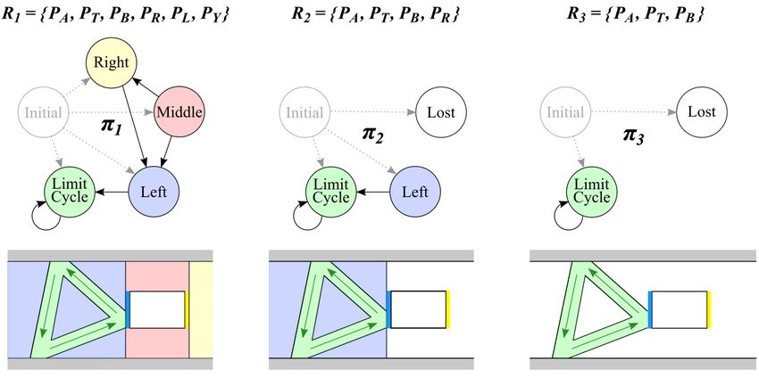
2       Nilles, Pervan, Berrueta, et al.

individual agents. In fact, micro-scale locomotion is often a direct consequence
of the fixed or low degree-of-freedom morphology of the robot, suggesting that
direct co-design of robots and their motion strategies may be necessary [4]. The
work presented in this manuscript provides the beginning of a theory of task-
centered robot design, used to devise micro-robot morphology and propulsion
mechanisms. In order to inform the design of task-capable micro-robotic plat-
forms, we analyze the information requirements of tasks [7].
    We focus on the task of micromanipulation with micro-robots, a fundamen-
tal task underlying more complex procedures such as drug delivery and cell
transplantation [13]. In this paper, we investigate micro-robot motion strategies
that explicitly use boundary interactions: the robot’s action when it encounters
an environment boundary. Identifying minimal information requirements in this
setting is essential for reasoning about robot performance, and is also a first step
toward automating co-design of robots and their policies. In Section 2, we define
abstract yet physically motivated models, aiming to roughly cover an interesting
set of possible micro-robot realizations. Section 3 motivates our task of interest
and our assumptions. In Section 4, we compare several robot designs and state
results on requirements for task completion, with respect to controller complex-
ity, sensor power, and onboard memory. Finally in Section 5 we state results for
the robustness of the periodic trajectories used in the hierarchical controller.

1.1   Background and Related Work

The scientific potential of precise manipulation at microscopic scales has been
appreciated for close to a century [5]. As micro/nano-robots have become in-
creasingly sophisticated, biomedical applications such as drug delivery [13] and
minimally-invasive surgery [21] have emerged as grand challenges in the field [25].
    To formally analyze the information requirements of planar micromanipula-
tion, we deliberately abstract many physically-motivated actuators and sensors,
such as odometry, range-sensing, differential-drive locomotion, and others. Ad-
ditionally, similar to the work in [7], we avoid tool-specific manipulation by
purposefully abstracting robot-object contacts in an effort to be more general.
However, we focus on collision-based manipulation instead of push-based. Recent
publications have illustrated the value of robot-boundary collisions in generating
reliable and robust robot behaviors [11,14,19]. Thus, through deliberate abstrac-
tion we develop and analyze a model of collision-based micromanipulation that
can serve as a test-bed for micro-robotic designs.
    Despite substantial advances in micro-robotics, agents at micro/nano length-
scales face fundamental difficulties and constraints. For one, as robots decrease
in size and mass, common components such as motors, springs and latches ex-
perience trade-offs in force/velocity generation that limit their output and con-
strain the space of feasible mechanical designs [9]. Furthermore, battery capac-
ities and efficiencies [16], as well as charging and power harvesting [6], experi-
ence diminishing performance at small scales, which restrict electrical designs of
micro-machines. These limitations collectively amount to a rebuke of tradition-
ally complex robotic design at the length-scales of interest, and suggest that a
Information Requirements of Collision-Based Micromanipulation 3
minimalist approach may be necessary. The minimal approach to robot design
asks, “what is the most simple robot that can accomplish a given task?”
Minimalist approaches to microrobot design often exploit the close relation-
ship between morphology and computation. For example, a DNA-based nano-
robot is capable of capturing and releasing molecular payloads in response to
a binary stimulus [8]. The inclusion of a given set of sensors or actuators in a
design can enable robotic agents to sidestep complex computation and planning
in favor of direct observation or action. Alternatively, in top-down approaches
the formulation of high-level control policies can guide the physical design of
robots [17]. While many approaches have seen success in their respective do-
mains, the problem of optimizing the design of a robot subject to a given task
has been shown to be NP-hard [18].
Due to information constraints, designing control policies for minimal robots
remains a challenge. In order to achieve complex tasks, controllers are often hand-
tuned to take advantage of the intrinsic dynamics of the system. For example,
in [1,2] the authors show that one can develop controllers for minimal agents
(solely equipped with a clock and a contact sensor) that can achieve spatial
navigation, coverage, and localization by taking advantage of the details of the
agents’ dynamics. Hence, in order to develop control strategies amenable to the
constraints of such robots, one requires substantial analytical understanding of
the capabilities of minimal robots.
A unifying theory of robotic capabilities was established in [15]. The authors
develop an information-based approach to analyzing and comparing different
robot designs with respect to a given task. The key insight lies in distilling the
minimal information requirements for a given task and expressing them in an
appropriately chosen information space for the task. Then, as long as we are ca-
pable of mapping the individual information histories of different robot designs
into the task information space, the performance of robots may be compared.
Our main contribution to this body of work is a novel demonstration of the ap-
proach in [15] to an object manipulation task. Additionally, we use a hierarchical
approach to combine the resulting high-level task completion guarantees with
results on the robustness of low-level controllers.
2 Model and Definitions
Here we introduce relevant abstractions for characterizing robots generally, as
well as their capabilities for given tasks. We largely follow from the work of [12,15].
2.1 Primitives and Robots
In this work, a robot is modelled as a point in the plane; this model has obvious
limitations, but captures enough to be useful for many applications, especially
in vitro where the robot workspace is often a thin layer of fluid. Hence, its
configuration space is X ⊆ SE(2), and its configuration is represented as (x, y, θ).
The robot’s environment is E ⊆ R2 , along with a collection of lines representing
boundaries; these may be one-dimensional “walls” or bounded polygons. The
environment may contain objects that will be static unless acted upon.4 Nilles, Pervan, Berrueta, et al.
Following the convention of [15], we define a robot through sets of primitives.
A primitive, Pi , defines a “mode of operation” of a robot, and is a 4-tuple Pi =
(Ui , Yi , fi , hi ) where Ui is the action set, Yi is the observation set, fi : X ×Ui → X
is the state transition function, and hi : X × Ui → Yi is the observation function.
Primitives may correspond to use of either a sensor or an actuator, or both if their
use is simultaneous (see [12] for examples). We will model time as proceeding in
discrete stages. At stage k the robot occupies a configuration xk ∈ X, observes
sensor reading yki ∈ Yi , and chooses its next action uik ∈ Ui for each i primitive in
its set. A robot may then be defined as a 5-tuple R = (X, U, Y, f, h) comprised of
the robot’s configuration space in conjunction with the elements of the primitives
4-tuples. With some abuse of notation, we occasionally write robot definitions as
R = {P1 , ..., PN } when robots share the same configuration space to emphasize
differences between robot capabilities.
2.2 Information Spaces
A useful abstraction to reason about robot behavior in the proposed frame-
work is the information space (I-space). Information spaces are defined accord-
ing to actuation and sensing capabilities of robots, and depend closely on the
robot’s history of actions and measurements. We denote the history of actions
and sensor observations at stage k as (u1 , y1 , . . . , uk , yk ). The history, com-
bined with initial conditions η0 = (u0 , y0 ), yields the history information state,
ηk = (η0 , u1 , y1 , . . . , uk , yk ). In this framework, initial conditions may either be
the exact starting state of the system, or a set of possible starting states, or a
prior belief distribution. The collection of all possible information histories is
known as the history information space, Ihist . It is important to note that a
robot’s history I-space is intrinsically defined by the robot primitives and its
initial conditions. Hence, it is not generally fruitful to compare the information
histories of different robots.
Derived information spaces should be constructed to reason about the capa-
bilities of different robot designs. A derived I-space is defined by an information
map κ : Ihist → Ider that maps histories in the history I-space to states in the
derived I-space Ider . Mapping different histories to the same derived I-space al-
lows us to directly compare different robots. The exact structure of the derived
I-space depends on the task of interest; an abstraction must be chosen that al-
lows for both meaningful comparison of the robots as well as determination of
task success.
In order to be able to compare robot trajectories within the derived I-space,
we introduce an information preference relation to distinguish between derived
information states [15]. We discriminate these information states based on a
distance metric to a given goal region IG ⊆ Ider which represents success for a
task. Using a relation of this type we can assess “preference” over information
states, notated as κ(η (1) ) κ(η (2) ) if an arbitrary η (2) is preferred over η (1) .
2.3 Robot Dominance
Extending on the definition of information preference relations in the previous
section, we can define a similar relation to compare robots. Here, we defineInformation Requirements of Collision-Based Micromanipulation 5
Fig. 1: (a) A rectangular object in a long corridor that can only translate to the
left or right, like a cart on a track. The robot’s task is to move the object into
the green goal region. (b) The robot, shown in green, executes a trajectory in
which it rotates the same relative angle each time it collides.
a relation that captures a robot’s ability to “simulate” another given a policy.
Policies are mappings π from an I-space to an action set: the current information
state determines the robot’s next action. We additionally define a function F
that iteratively applies a policy to update an information history. The updated
history I-state is given by ηm+k = F m (ηk , π, xk ), where xk ∈ X.
Definition 1. (Robot dominance from [15]) Consider two robots with a task
specified by reaching a goal region IG ⊆ Ider :
R1 = (X (1) , U (1) , Y (1) , f (1) , h(1) )
R2 = (X (2) , U (2) , Y (2) , f (2) , h(2) ).
(1) (2) (1)
Given I-maps κ1 : Ihist → Ider and κ2 : Ihist → Ider , if for all: η (1) ∈ Ihist
(2)
and η (2) ∈ Ihist for which κ1 (η (1) ) κ2 (η (2) ); and u(1) ∈ U (1) ; there exists a
(2)
policy, defined as π2 : Ihist → U (2) , generating actions for R2 such that for all
(1) (1)
x ∈X consistent with η (1) and all x(2) ∈ X (2) consistent with η (2) , there
exists a positive integer l such that
κ1 (η (1) , u(1) , h(1) (x(1) , u(1) )) κ2 (F l (η (2) , π2 , x(2) ))
then R2 dominates R1 under κ1 and κ2 , denoted R1 E R2 . If both robots can
simulate each other (R1 E R2 and R2 E R1 ), then R1 and R2 are equivalent,
denoted by R1 ≡ R2 . Lastly, we introduce the following lemma:
Lemma 1. (from [15]) Consider three robots R1 , R2 , and R3 and an I-map κ.
If R1 E R2 under κ, we have:
(a) R1 E R1 ∪ R3 (adding primitives never hurts);
(b) R2 ≡ R2 ∪ R1 (redundancy does not help);
(c) R1 ∪ R3 E R2 ∪ R3 (no unexpected interactions).
3 Manipulating a Cart in a Long Corridor
We begin our analysis of the information requirements of micro-scale object
manipulation by introducing a simple, yet rich, problem of interest. Consider a
long corridor, containing a rectangular object, as shown in Fig. 1(a). The object
may only translate left or right down the corridor, and cannot translate toward
the corridor walls or rotate. We can abstract this object as a cart on a track;6 Nilles, Pervan, Berrueta, et al.
physically, such one-dimensional motion may arise at the micro-scale due to
electromagnetic forces from the walls of the corridor, from fluid effects, or from
direct mechanical constraints. The task for the robot is then to manipulate the
object into the goal region (green-shaded area in Fig. 1(a)). We believe that this
simplified example will illustrate several interesting trade-offs in the sensing,
memory, and control specification complexity necessary to solve the problem.
On its own merits, this task solves the problem of directed transport, and can be
employed as a useful component in larger, more complex microrobotic systems.
To break the symmetry of the problem, we assume that the object has at
least two distinguishable sides (left and right). For example, the two ends of the
object may emit chemical A from the left side and chemical B from the right side.
The robot may be equipped with a chemical comparator that indicates whether
the robot is closer to source A or source B (with reasonable assumptions on
diffusion rates). The object may have a detectable, directional electromagnetic
field. All these possible sensing modalities are admissible under our model. We
also assume that the dimensions of the corridor and the object are known and
will be used to design the motion strategy of the robot—often a fair assumption
in laboratory micro-robotics settings.
Here, we investigate the requirements of minimal strategies for object manip-
ulation, given the constraints of micro-robotic control strategies. In the spirit of
minimality, we aim to tailor our low-level control policies to the natural dynam-
ical behaviors of our system prior to the specification of increasingly abstract
control policies. To this end, we have chosen to study “bouncing robots,” which
have been shown to exhibit several behaviors, such as highly robust limit cy-
cles, chaotic behavior, and large basins of attraction [1,14,22]. Once discovered,
these behaviors can be chained together and leveraged towards solving robotic
tasks such as coverage and localization without exceedingly complex control
strategies [3]. The key insight in this paper is that by taking advantage of spon-
taneous limit cycles in the system dynamics, trajectories can be engineered that,
purely as a result of the incidental collisions of the robot, manipulate objects
in the robot’s environment. Figure 1(b) shows an example of such a trajectory
constructed from iterative executions of the natural cyclic behavior of the bounc-
ing robots. A detailed analysis of this dynamical system and its limit cycles are
presented in Section 5.
4 A Formal Comparison of Several Robot Designs
In order to achieve the goal of manipulating an object in a long corridor, we will
introduce several robot designs and then construct policies that each robot might
use to accomplish the task. Particularly, these robots were designed to achieve
the limit cycle behavior of bouncing robots, and to use this cyclic motion pattern
to push the object in a specified direction.
Prior to describing the robot designs, we introduce the relevant primitives
that will be used to construct the robots. Figure 2 shows four robotic primitives
taken directly from [15] (PA , PL , PT , and PR ) and two additional primitives
defined for the proposed task (PB and PY ). The primitive PA describes a ro-
tation relative to the local reference frame given an angle uA . PL correspondsInformation Requirements of Collision-Based Micromanipulation 7
Fig. 2: Simple robotic behaviors called primitives. PA is a local rotation, PT is
a forward translation to an obstacle, PL is a forward translation a set distance,
PR is a range sensor, PB senses the color blue, and PY senses the color yellow.
to a forward translation over a chosen distance uL , and PT carries out forward
translation in the direction of the robot’s heading until it reaches an obstacle.
In addition to these actuation primitives, we define PR as a range sensor where
yR is the distance to whatever is directly in front of the robot. For the 4-tuple
specification of these primitives we refer the reader to [15]. The chosen prim-
itives were largely selected based on their feasibility of implementation at the
micro-scale, as observed in many biological systems [22,10].
To differentiate different facets of the object being manipulated, we employ
two primitives that are sensitive to the signature of each side of the target.
PB is a blue sensor that measures yB = 1 if the color blue is visible (in the
geometric sense) given the robot’s configuration (x, y, θ), and PY is a yellow
sensor outputting yY = 1 if the color yellow is visible to the robot. More formally,
we define PB = (0, {0, 1}, fB , hB ) and PY = (0, {0, 1}, fY , hY ), where fB and
fY are trivial functions always returning 0, and the observation functions hB
and hY return 1 when the appropriate signature is in front of the robot. We
deliberately make the “blue” and “yellow” sensors abstract since they should be
thought of as placeholders for any sensing capable of breaking the symmetry of
the manipulation task, such as a chemical comparator, as discussed in Section 3.
These six simple primitives, shown in Fig. 2 can be combined in different ways
to produce robots of differing capabilities. Notably, here we develop modular
subroutines and substrategies that allow us to develop hierarchical robot designs,
enabling straightforward analysis of their capabilities. The corresponding task
performance and design complexity trade-offs between our proposed robots and
their constructed policies are explored in the following subsections.
4.1 Robot 0: Omniscient and Omnipotent
In many reported examples in micro-robot literature, the robots—as understood
through the outlined framework—are not minimal. Often, instead of grappling
with the constraints of minimal on-board computation, designers make use of8 Nilles, Pervan, Berrueta, et al.
Fig. 3: The Limit Cycle strategy uses the primitive PT , which moves forward
until coming into contact with an object, and PA , which rotates relative to the
robot heading. Once a limit cycle is completed, the count variable is incremented.
external sensors and computers to observe micro-robot states, calculate opti-
mal actions, and actuate the micro-robots using external magnetic fields, sound
waves, or other methods [13,23,24]. Given the prevalence of such powerful robots
in the literature, we introduce a “perfect” robot to demonstrate notation and
compare to the minimal robots we present in the following sections.
We can specify the primitive for an all-capable robot as PO = (SE(2), SE(2)×
SE(2), fO , hO ), where the action set UO is the set of all possible positions and
orientations in the plane, and the observation set YO is the set of all possible
positions and orientations in the plane of both the robot and the object. The
state transition function is fO (x, u) = (x + uOx ∆tk , y + uOy ∆tk , θ + uOθ ∆tk )
where uOx , uOy , uOθ ∈ R, and ∆tk ∈ R+ is the time step corresponding to
the discrete amount of time passing between each stage k. The observation
function outputs the current configurations of the robot and object. A robot
with access to such a primitive (i.e., through external, non-minimal computing)
would be able to simultaneously observe themselves and the object anywhere
in the configuration space at all times and dexterously navigate to any location
in the environment. Given that the configuration space of the robot is some
bounded subset X of SE(2), the robot definition for this omniscient robot is
R0 = (X, SE(2), SE(2) × SE(2), fO , hO ). Since all robots employed in the task
of manipulating the cart in the long corridor share the same bounded configu-
ration space X ⊆ SE(2), we also can define this robot using R0 = {PO }. We
use this alternative notation for robot definitions as it is less cumbersome and
highlights differences in capabilities. While it is clear that such a robot should
be able to solve the task through infinitely many policies, we provide an example
of such a policy π0 that completes the task in Algorithm 2 in the Appendix.
4.2 Robot 1: Complex
The underlying design principle behind each of the following minimal robotic
designs is modularity. We use a hierarchical control approach: at the highest
level, we have a few spatio-temporal states (see Fig. 4). In each state, we use
our available primitives to develop subroutines corresponding to useful behaviorsInformation Requirements of Collision-Based Micromanipulation 9
such as wall following, measuring distance to an object, and orienting a robot in
the direction of the blue side of the cart. These subroutines are specified in the
Appendix. Moreover, through these subroutines we construct substrategies that
transition the robots between states, such as moving from the right hand side of
the object to the left hand side. We represent the complete robot policy πi as a
combination of these substrategies in the form of a finite state machine (FSM).
The key substrategy that enables the success of our minimal robot designs is
the Limit Cycle substrategy (shown in Fig. 3), which requires two primitives, PA
and PT , to perform. This substrategy is enabled by the fact that these bouncing
robots converge to a limit cycle for a non-zero measure set of configurations
(as shown in Section 5). All other substrategies employed in the design of our
robots serve the purpose of positioning the robot into a configuration where it
is capable of carrying out the limit cycle substrategy.
Hence, we define our robot as R1 = {PA , PT , PB , PR , PL , PY }, which makes
use of all six of the primitives shown in Fig. 2. Its corresponding policy π1 , as
represented by an FSM, is shown in Fig. 4. The details describing this policy are
in Algorithm 3 in the Appendix. We highlight that through this policy the robot
is capable of succeeding at the task from any initial condition. The substrategy
structure of the FSM—containing Initial, Left, Right, Middle and Limit Cycle
states—corresponds to different configuration domains that the robot may find
itself in as represented by the shaded regions in Fig. 4. Due to the structure of
the FSM and the task at hand, if the robot is in the Limit Cycle state it will
eventually succeed at the task. Finally, although we allocate memory for the
robot to track its success through a variable count (as seen in the substrategy
in Fig. 3) the robot does not require memory to perform this substrategy and
we have only included it for facilitating analysis.
4.3 Robot 2: Simple
Robot 2, defined as R2 = {PA , PT , PB , PR }, is comprised of a subset of the
primitives from R1 . As a result, it is not capable of executing all of the same
motion plans as R1 . As Fig. 4 shows, R2 can enter its Limit Cycle substrategy if
it starts on the left side of the object, but otherwise it will get lost. The Initial
state uses sensor feedback to transition to the substrategy the robot should use
next. The Lost state is distinct from the Initial state—once a robot is lost, it
can never recover (in this case, the robot will move until it hits a wall and then
stay there for all time). More details on policy π2 and the specific substrategies
that R2 uses can be found in Algorithm 4 in the Appendix.
4.4 Robot 3: Minimal
Robot 3, R3 = {PA , PT , PB }, contains three robotic primitives, which are a
subset of the primitives of R1 and R2 . Under policy π3 (detailed in Algorithm 5 in
the Appendix), this robot can only be successful at the task if it initializes in the
Limit Cycle state, facing the correct direction. Otherwise, the robot will never
enter the limit cycle. Such a simple robot design could be useful in a scenario
when there are very many “disposable” robots deployed in the system. Even if
only a small fraction of these many simple robots start out with perfect initial10 Nilles, Pervan, Berrueta, et al.
Fig. 4: (Left) A complex robot (composed of 6 primitives) can successfully
achieve its goal no matter its initial conditions. (Middle) A simple robot (com-
posed of 4 primitives) can only be successful if its initial conditions are on the
left side of the object. (Right) A minimal robot (composed of 3 primitives) can
only be successful if its initial conditions are within the range of the limit cycle.
conditions, the goal would still be achieved. Despite the apparent simplicity of
such a robot, we note that R3 (along with all other introduced designs) is capable
of determining whether or not it is succeeding at the task or whether it is lost
irreversibly. Such capabilities are not by any means trivial, but are included in
the robot designs for the purposes of analysis and comparison.
4.5 Comparing Robots
We will compare the four robots introduced in this section, R0 , R1 , R2 , and
R3 . In order to achieve this we must first specify the task and derived I-space in
which we can compare the designs. The chosen derived I-space is Ider = Z+ ∪{0}.
Specifically, it consists of counts of the Limit Cycle state (the count variable is
shown in Fig. 3 and in the algorithms in the Appendix). If we assume that after
each collision the robot pushes the object a distance , task success is equivalently
tracked in memory by count up to a scalar.
We express the goal for the task of manipulating the cart in a long corridor
as IG ⊆ Ider , where IG is an open subset of the nonnegative integers. In this
set up, as illustrated in Fig. 1(a), the robot must push the object some N times,
corresponding to a net distance traveled, to succeed. More formally, we express
our information preference relation through the indicator 1G (η) corresponding
to whether a derived information history is within the goal region IG , thereby
inducing a partial ordering over information states. Hence, the likelihood of
success of any of the proposed robot designs (excluding R0 ) is solely determined
by their initialization, and the region of attraction of the limit cycle behavior
for the bouncing robots, which will be explored in more detail.
Comparing R1 , R2 , and R3 The comparison of robots R1 , R2 , and R3
through the lens of robot dominance is straightforward given our modular robotInformation Requirements of Collision-Based Micromanipulation 11
designs. Since R1 and R2 are comprised of a superset of the primitives of R3 , they
are strictly as capable or more capable than R3 , as per Lemma 1(a). Therefore,
we state that R1 and R2 dominate R3 , denoted by R3 E R1 , and R3 E R2 .
Likewise, using the same lemma, we can see that R2 E R1 . This is to say that for
the task of manipulating the cart along the long corridor R1 should outperform
R2 and R3 , and that R2 should outperform R3 .
While the policies for each robot design are nontrivial, Fig. 4 offers intuition
for the presented dominance hierarchies. Effectively, if either R2 or R3 are ini-
tialized into their Lost state they are incapable of executing the task for all time.
Hence, it is the configuration space volume corresponding to the Lost state that
determines the robot dominance hierarchy.
(1) (2) (3)
Let η (1) ∈ Ihist , η (2) ∈ Ihist , η (3) ∈ Ihist , and define I-maps that return
the variable count stored in memory for each robot. The information preference
relation then only discriminates whether the information histories correspond to
a trajectory reaching IG ⊆ Ider —in other words, whether a robot achieves the
required N nudges to the object in the corridor. Note that since there is no time
constraints to the task, this number is arbitrary and only relevant for tuning to
the length-scales of the problem. Thus, the dominance relations outlined above
follow from the fact that for non-zero volumes of the configuration space there
exists no integer l for which κ1 (η (1) ) κ2 (F l (η (2) , π2 , x)). On the other hand
for all x ∈ X, κ2 (η (2) ) κ1 (F l (η (1) , π1 , x)). Through this same procedure we
can deduce the rest of the hierarchies presented in this section.
Comparing R0 and R1 To compare R0 and R1 we may continue with a
similar reachability analysis as in the previous subsection. We note that from any
x ∈ X, R1 and R0 are capable of reaching the object and nudging it. This means
that given that the domain X is bounded and information history states η (0) ∈
(0) (1)
Ihist , η (1) ∈ Ihist corresponding to each robot, there always exists a finite integer
l such that κ0 (η (0) ) κ1 (F l (η (1) , π1 , x)), and κ1 (η (1) ) κ0 (F l (η (0) , π0 , x)). So
we have that R1 E R0 and R0 E R1 , meaning that R1 ≡ R0 . Thus, R0 and R1
are equivalently capable of performing the considered task.
It is important to note that despite the intuition that R0 is more “powerful”
than R1 in some sense, for the purposes of the proposed task that extra power
is redundant. However, there are many tasks where this is would not be the case
(e.g., moving the robot to a specific point in the plane).
Comparing R0 , R2 and R3 Lastly, while the relationship between R0 and
the other robot designs is intuitive, we must introduce an additional lemma.
Lemma 2. (Transitive property) Given three robots R0 , R1 , R2 , if R2 E R1 and
R1 ≡ R0 , then R2 E R0 .
Proof. The proof of the transitive property of robot dominance comes from the
definition of equivalence. R1 ≡ R0 means that the following statements are
simultaneously true: R1 E R0 and R0 E R1 . Thus, this means that R2 E R1 E R0 ,
which implies that R2 E R0 , concluding the proof.
Using this additional lemma, we see that R2 E R0 , and R3 E R0 , as expected.
Hence, we have demonstrated that minimal robots may be capable of executing
complex strategies despite the constraints imposed by the micro-scale domain.12 Nilles, Pervan, Berrueta, et al.
Fig. 5: (a) The three types of bounce rules considered. The top row depicts fixed
bounce rules, where the robot leaves the boundary at a fixed angle regardless
of the incoming trajectory. The second row shows fixed monotonic bounce rules
preserving the horizontal direction of motion but keep the absolute angle between
the boundary and the outgoing trajectory fixed. The third row shows relative
bounce rules rotating the robot through an angle relative to its previous heading.
(b) The geometric setup for analyzing dynamics of triangular trajectories formed
by repeated single-instruction relative bounce rules.
Minimality in micromanipulation is in fact possible when robot designs take
advantage of naturally occurring dynamic structures, such as limit cycles. In
the following sections we discuss the necessary conditions for establishing such
cycles, as well as the robustness properties of limit cycle behavior, which are
important for extending this work to less idealized and deterministic settings.
5 Feasibility and Dynamics of Cyclic Motion Strategies
In this section we will derive and analyze limit cycle motion strategies that can be
used to manipulate objects through incidental collisions. The goal is to engineer
robust patterns in the robot’s trajectory that are useful for this task. When
looking to move an object down the corridor, three boundaries are present: the
two walls of the corridor, and the object itself. An ideal motion strategy would
use collisions with the two walls to direct the robot to collide with the object
in a repeatable pattern. Is it possible to do so with a single instruction to the
robot that it repeats indefinitely, every time it encounters a boundary? This
single-instruction strategy would lend itself well to the design of a micro-robot,
so that the robot robustly performs the correct boundary interaction each time.
We consider three types of boundary actions, as seen in Fig. 5(a). The first
and second types (fixed bounce rules) could be implemented through alignment
with the boundary (mechanical or otherwise) such that forward propulsion oc-
curs at the correct heading. This measurement and reorientation can be done
compliantly, and does not necessarily require traditional onboard measurement
and computation. See, for example, similar movement profiles of microorgan-
isms resulting from body morphology and ciliary contact interactions [10,22].
The third type of boundary interaction (relative bounce rule) requires a rotation
relative to the robot’s prior heading, implying the need for rotational odometry
or a fixed motion pattern triggered upon collision.
Here, we analyze the relative power of these actions for the task of pushing
an object down a hallway, without considering the broader context of initialInformation Requirements of Collision-Based Micromanipulation 13
conditions or localization, which were considered in Section 4. Particularly, we
consider the system of the robot, hallway and object as a purely dynamical
system, to establish the feasibility of trajectories resulting from minimal policies.
For the rest of this section, suppose that the bouncing robot navigates in a
corridor with parallel walls and a rectangular object as described in Section 3.
Proposition 1. For all bouncing robot strategies consisting of a single repeated
fixed bounce rule, there does not exist a strategy that would result in a triangular
trajectory that makes contact with the rectangular object.
Proof. A fixed bounce rule in this environment will result in the robot bouncing
back and forth between the two parallel walls forever after at most one con-
tact with the object. A monotonic fixed bounce rule would result in the robot
bouncing down the corridor away from the object after at most one contact.
Remark 1. The feasibility of fixed (monotonic) bounce rule strategies in envi-
ronments without parallel walls is unknown and possibly of interest.
Proposition 2. There exist an infinite number of strategies consisting of two
fixed bounce rules that each result in a triangular trajectory that makes contact
with the rectangular object. The robot must also be able to distinguish the object
from a static boundary, or must know its initial conditions.
Proof. Geometrically, an infinite number of triangles exist that can be executed
by a robot with the choice between two different fixed bounce rules. It is nec-
essary that the robot be able to determine when it has encountered the first
corridor wall during its cycle, in order to switch bounce rules to avoid the sit-
uation described in the proof of Proposition 1. One sufficient condition is that
the robot knows the type of boundary at first contact, and has one bit of mem-
ory to track when it encounters the first corridor wall and should switch actions.
Equivalently, a strategy could use a sensor distinguishing the object from a static
boundary at collision time, along with one bit of memory.
Proposition 3. There exists a strategy consisting of a single repeated relative
bounce rule that results in a triangular trajectory that makes contact with the
rectangular object. Moreover, this strategy is robust to small perturbations in the
rotation θ and the initial angle α.
Proof. See Fig. 5(b) for the geometric setup. Here we will provide exact expres-
sions for the quantities x, y and z as a function of the initial conditions, position,
and orientation of the robot on its first collision with the object.
First assume xk is given, as the point of impact of the robot with the object
at stage k. Let α be the angle indicated in Fig. 5(b), the angle between the
incoming trajectory at xk and the object face. Then, using simple trigonometry,
y = (` − xk ) tan(π − θ − α) where θ is the interior angle of the robot’s rotation.
To create an equiangular triangle, θ = π3 , but we will leave θ symbolic for now
to enable sensitivity analysis. To compute z, we consider the horizontal offset
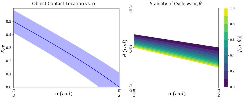
due to the transition from the top to the bottom of the hallway. This leads to14 Nilles, Pervan, Berrueta, et al.
Fig. 6: (Left) The location of the impact on the object is nearly a linear function
of α for θ = π3 ±0.1. Only the counterclockwise cycle is shown; the clockwise cycle
follows from symmetry. (Right) The Jacobian of this system indicates robustness
to small perturbations in θ (white regions represent instability or infeasibility).
z = y + ` cot( 3π
2 − 2θ − α). Finally, we can compute the coordinate of where the
robot will return to the object, xk+3 = z tan( 3π
2 − α − 3θ). Solving for the fixed
point of this dynamical system, xF P = xk = xk+3 gives
tan(α + θ) − tan(α + 2θ)
xF P = ` .
tan(α + θ) − tan(α + 3θ)
Note that this xF P expression is not valid for all values of (α, θ), but only for
values leading to inscribed triangles in the environment such that xF P > 0.
For θ = π3 , Fig. 6 (Left) shows the location of the fixed point as a function
of the angle α, indicating that an infinite number of stable cycles exist for this
motion strategy, and every point of the object in the bottom half of the corridor
is contactable with counterclockwise cycles. The top half of the object can be
reached using clockwise cycles.
Since xk+3 = F (xk , α, θ) is linear in xk , the Jacobian is J = − tan(α +
θ) tan(α+3θ − π2 ). Figure 6 (Right) shows the value of the Jacobian as a function
of α and θ. All the shaded regions have an absolute value less than one, indicating
robustness to small perturbations of α and θ over a large domain.
Remark 2. We note that Propositions 2 and 3 are equivalent in terms of memory
requirements, both requiring the robot to “remember” either its previous heading
or its previous bounce rule at each stage of the strategy. However, the fixed
bounce strategy implies that the robot has more knowledge of its surroundings
than the relative bounce strategy, as it must measure the plane of the boundary it
encounters and orient itself appropriately. The relative bounce strategy requires
only information within the robot’s own reference frame.
6 Conclusion
In this paper, we have designed robust motion strategies for minimal robots that
have great promise for micromanipulation. We have also analyzed the informa-
tion requirements for task success, compared the capabilities of four different
robot designs, and found that minimal robot designs may still be capable ofInformation Requirements of Collision-Based Micromanipulation 15
micromanipulation without the need for external computation. While our exam-
ple of a rectangular obstacle in a corridor is simple, we think of this as robust
directed transport, a key building block for future work.
6.1 Future Directions
The setting of micro-robotics provides motivation for the approach we have laid
out in this work. At the micro-scale, coarse high-level controllers that can be
applied to a collection of many micro-robots are easier to implement than fine-
grained individual controllers. This requires formal reasoning about all possible
trajectories, in order to funnel the system into states that allow for task com-
pletion, as was illustrated in this work. In order to be more applicable in the
micro-robotics domain, it will be important to extend the approach to multi-
ple agents, as well as scenarios subject to noise. While our strategies passively
provide some noise tolerance by virtue of the limit cycle region of attraction,
there is much work to be done on more concrete applications to characterize and
account for sensing and actuation noise.
Outside of our particular model and application, this work has implications
for the future of robot behavior and design. Often, derived I-states are designed
to infer information such as the set of possible current states of the robot, or the
set of possible states that the robot could have previously occupied. In this work,
we focus on derived I-spaces that encode information about what will happen to
the robot under a given strategy. With these forward-predictive derived I-spaces,
we encode a high density of task-relevant information into a few-state symbolic
abstraction. By making use of such abstractions, minimal agents may be endowed
with a passively predictive capacity leading to greater task-capability.
More broadly, this work provides an exciting glimpse toward more automated
analysis, through a combination of system identification techniques, hybrid sys-
tems theory, and I-space analysis. Coarse-grained sensors provide an avenue for
discretization useful for hierarchical control; such an approach is increasingly
needed as our robotic systems become more data-driven. Such a unified ap-
proach may be able to simultaneously identify coarse-grained system dynamics,
predict their task-capabilities, and design fine-tuned control strategies.
References
1. T. Alam, L. Bobadilla, and D. A. Shell. Minimalist robot navigation and coverage
using a dynamical system approach. In IEEE Int. Conf. Rob. Comp., 2017.
2. T. Alam, L. Bobadilla, and D. A. Shell. Space-efficient filters for mobile robot
localization from discrete limit cycles. IEEE Rob. Auto. Lett., 3(1):257–264, 2018.
3. A. Bayuelo, T. Alam, L. Bobadilla, L. F. Niño, and R. N. Smith. Computing
feedback plans from dynamical system composition. In IEEE Int. Conf. Auto. Sci.
Eng., pages 1175–1180, 2019.
4. A. Censi. A mathematical theory of co-design. Technical report, September 2016.
Conditionally accepted to IEEE Trans. Rob.
5. R. Chambers, H. B. Fell, and W. B. Hardy. Micro-operations on cells in tissue
cultures. Proc. Royal Soc. of London., 109(763):380–403, 1931.
6. J. Ding, V. R. Challa, M. G. Prasad, and F. T. Fisher. Vibration Energy Harvesting
and Its Application for Nano- and Microrobotics. Springer, New York, NY, 2013.16 Nilles, Pervan, Berrueta, et al.
7. B. R. Donald, J. Jennings, and D. Rus. Information invariants for distributed
manipulation. Int. J. Rob. Res., 16(5):673–702, 1997.
8. S. M. Douglas, I. Bachelet, and G. M. Church. A logic-gated nanorobot for targeted
transport of molecular payloads. Science, 335(6070):831–834, 2012.
9. M. Ilton, M. S. Bhamla, X. Ma, S. M. Cox, L. L. Fitchett, Y. Kim, J. Koh, D. Kr-
ishnamurthy, C. Kuo, F. Z. Temel, A. J. Crosby, M. Prakash, G. P. Sutton, R. J.
Wood, E. Azizi, S. Bergbreiter, and S. N. Patek. The principles of cascading power
limits in small, fast biological and engineered systems. Science, 360(6387), 2018.
10. Vasily Kantsler, Jörn Dunkel, Marco Polin, and Raymond E Goldstein. Ciliary
contact interactions dominate surface scattering of swimming eukaryotes. Proc.
Natl. Acad. Sci., 110(4):1187–1192, 2013.
11. J. Kim and D. A. Shell. A new model for self-organized robotic clustering: Under-
standing boundary induced densities and cluster compactness. In IEEE Int. Conf.
Rob. Auto. (ICRA), pages 5858–5863, May 2015.
12. S. M. LaValle. Planning Algorithms. Cambridge University Press, USA, 2006.
13. J. Li, B. Esteban-Fernández de Ávila, W. Gao, L. Zhang, and J. Wang. Mi-
cro/nanorobots for biomedicine: Delivery, surgery, sensing, and detoxification. Sci.
Rob., 2(4), 2017.
14. A. Q. Nilles, Y. Ren, I. Becerra, and S. M. LaValle. A visibility-based approach
to computing nondeterministic bouncing strategies. Int. Work. Alg. Found. Rob.,
Dec. 2018.
15. J. M. O’Kane and S. M. LaValle. Comparing the power of robots. Int. J. Rob.
Res., 27(1):5–23, 2008.
16. J. F. M. Oudenhoven, L. Baggetto, and P. H. L. Notten. All-solid-state lithium-ion
microbatteries: A review of various three-dimensional concepts. Adv. Energy Mat.,
1(1):10–33, 2011.
17. A. Pervan and T. D. Murphey. Low complexity control policy synthesis for em-
bodied computation in synthetic cells. Int. Work. Alg. Found. Rob., Dec. 2018.
18. F. Z. Saberifar, J. M. O’Kane, and D. A. Shell. The hardness of minimizing design
cost subject to planning problems. Int. Work. Alg. Found. Rob., Dec. 2018.
19. W. Savoie, T. A. Berrueta, Z. Jackson, A. Pervan, R. Warkentin, S. Li, T. D.
Murphey, K. Wiesenfeld, and D. I. Goldman. A robot made of robots: Emergent
transport and control of a smarticle ensemble. Sci. Rob., 4(34), 2019.
20. M. Sitti, H. Ceylan, W. Hu, J. Giltinan, M. Turan, S. Yim, and E. Diller.
Biomedical applications of untethered mobile milli/microrobots. Proc. of IEEE,
103(2):205–224, Feb. 2015.
21. F. Soto and R. Chrostowski. Frontiers of medical micro/nanorobotics: in vivo
applications and commercialization perspectives toward clinical uses. Front. in
Bioeng. and Biotech., 6:170–170, Nov. 2018.
22. S. E. Spagnolie, C. Wahl, J. Lukasik, and J. Thiffeault. Microorganism billiards.
Phys. D, 341:33–44, 2016.
23. T. Xu, J. Yu, X. Yan, H. Choi, and L. Zhang. Magnetic actuation based motion
control for microrobots: An overview. Micromachines, 6(9):1346–1364, Sept. 2015.
24. T. Xu, J. Zhang, M. Salehizadeh, O. Onaizah, and E. Diller. Millimeter-scale
flexible robots with programmable three-dimensional magnetization and motions.
Sci. Rob., 4(29), 2019.
25. G. Z. Yang, J. Bellingham, P. E. Dupont, P. Fischer, L. Floridi, R. Full, N. Jacob-
stein, V. Kumar, M. McNutt, R. Merrifield, B. J. Nelson, B. Scassellati, M. Taddeo,
R. Taylor, M. Veloso, Z. L. Wang, and R. Wood. The grand challenges of science
robotics. Sci. Rob., 3(14), 2018.Information Requirements of Collision-Based Micromanipulation 17
Appendix
Subroutines
We define how the subroutines introduced in Section 4 can be achieved. Sub-
routines for wall following (in a random direction) for uL steps, observing the
object yR , yB , yY , and orienting in the direction of the blue side of the object
are shown below, in Algorithm 1.
Algorithm 1 Subroutines
wall follow (input uL )
while PR (yR 6= ∞) (while the robot is not parallel to the wall)
PA (uA = φ) (rotate a small angle φ)
PL (uL ) (step forward a distance uL )
.
.
observe object (output yR , yB , yY )
inc = 0
while PB (yB = 0) and PY (yY = 0) and inc ≤ 360◦ (while neither yellow nor blue
. are detected, and the robot has
. not completed a full rotation)
PA (uA = φ) (rotate a small angle φ)
inc + +
if yB = 1 or yY = 1 (if blue or yellow are detected)
yR = PR (measure the distance to the color)
else
yR = ∞ (otherwise, return ∞ to encode ‘no color’)
.
.
aim toward blue ()
while PB (yB = 0) (while blue is not detected)
PA (uA = φ) (rotate a small angle φ)
For wall following, the robot continuously rotates a small angle (using the
PA primitive) until it detects that there is nothing in front of it (when the range
detecting primitive PR reads ∞), and is therefore facing a direction parallel to
the wall. Then the robot uses primitive PL to move forward uL steps.
For observing the object, the robot continuously rotates until it has either
detected the blue side of the object, detected the yellow side of the object, or
completed a full rotation. If it has detected a color, it records the distance to the
object and the color detected (if a color was detected). If the robot completes a
full rotation without detecting either color, it returns a range of ∞, to encode
that no color was found. It is possible to call a subset of measurements from this
subroutine, for example in Algorithm 3 the Middle substrategy only queries the
observe object() subroutine for yB and yY .18 Nilles, Pervan, Berrueta, et al.
For aiming toward blue, the robot will rotate in place (using PA ) until it
detects the color blue (using PB ).
Robot 0 Policy
Robot 0 uses the primitive PO , and requires knowledge of the width of the
channel, `, and the length of the object, 2s. First, in its initial state, it observes
its own position (xr , yr ) and the position of the object (xo , yo ). If the robot, xr ,
is to the left of object’s left edge, (xo − s) (where xo is the center of mass of
the object and s is half the length of the object), then the robot should execute
substrategy Left.
If robot is to the right of the object’s edge, it will go straight up, uOy = `/∆tk ,
to either the top wall of the channel, or the underside of the object (if the robot
happened to start below the object), and then move left, uOx = ((xo − s) −
xr )/∆tk , until it has passed the object. Then the robot transitions to the Left
substrategy.
In the Left substrategy, the robot translates to the left side of the object,
and then pushes it a set distance to the right. It increases the count variable
with each subsequent push.
Algorithm 2 Robot 0 Policy: π0
Requires
Primitive: PO
Parameters: s is half of the length of the object, ` is the width of the channel
.
Initial
count = 0
xr , yr , xo , yo = PO () (read the positions of the robot and the object)
if xr < (xo − s) (if the robot is to the left of the object’s left edge)
Switch to Left
else
PO (uOx = 0, uOy = `/∆tk ) (move up, until the object or wall)
PO (uOx = ((xo − s) − xr )/∆tk , uOy = 0) (move to the left of the object)
Switch to Left
.
.
Left
PO (uOx = ((xo − s) − xr )/∆tk , uOy = (yo − yr )/∆tk ) (go to the center of the
. left side of the object)
PO (uOx = /∆tk , uOy = 0) (push the object a distance of to the right)
count + +Information Requirements of Collision-Based Micromanipulation 19
Robot 1 Policy
Robot 1 uses the primitives PA , PT , PB , PR , PL , and PY , and requires knowledge
of the set of distances w from the object that allow the robot to fall into the
limit cycle. First, in its initial state, R1 measures the distance between it and
the object, and the color directly in front of it (if any). It uses this knowledge
to switch to a substrategy: either Limit Cycle, Left, Right, or Middle.
In the Limit Cycle substrategy, as shown in Fig. 3, the robot translates for-
ward, rotates, and repeats – continuously executing the limit cycle and counting
how many times it bumps the object forward.
In the Left substrategy, the robot orients itself so that it is facing the blue
side of the object, then switches to Limit Cycle, where it will translate toward
the object, rotate, and enter the limit cycle.
In the Right substrategy, R1 will measure the distance to the object yR old ,
move along the wall a small distance δ, then measure the distance to the object
again yR , and compare the two distances. If the distance to the object increased,
then the robot is moving toward the right and must turn around, using primitive
PA . Otherwise, the robot is moving toward the left, and will continue in that
direction until it detects the blue side of the object and switches to the Left
substrategy.
In the Middle substrategy, the robot is directly beneath or above the object,
and cannot tell which direction is which. It chooses a random direction to follow
the wall, until it detects either the blue or the yellow side of the object. If it
detects blue it switches to the Left substrategy, and if it detects yellow it switches
to the Right substrategy.20 Nilles, Pervan, Berrueta, et al.
Algorithm 3 Robot 1 Policy: π1
Requires
Primitives: PA , PT , PB , PR , PL , PY
Parameters: w is the range of distances that are attracted by the limit cycle
.
Initial
count = 0
yR , yB , yY = observe object() (read object distance and color)
if yB = 1 and yR ∈ w (if blue was detected at a distance in w)
Switch to Limit Cycle
else if yB = 1 and yR ∈ /w (if blue was detected at a distance not in w)
Switch to Left
else if yY = 1 (if yellow was detected)
Switch to Right
else
Switch to Middle
.
.
Limit Cycle
PT (translate forward to an obstacle)
PA (uA = θ) (rotate θ)
PT (translate forward to an obstacle)
PA (uA = θ) (rotate θ)
PT (translate forward to an obstacle)
PA (uA = θ) (rotate θ)
count + +
.
.
Left (bounce off of blue side of object)
aim toward blue()
Switch to Limit Cycle
.
.
Right (wall follow toward object)
yR old = observe object() (read object distance)
wall follow(uL = δ) (step forward a small distance δ)
yR = observe object() (read object distance)
if yR > yR old (if the distance to the object increased)
PA (uA = 180◦ ) (turn around)
while yB = 0 (while blue has not been detected)
wall follow(uL = δ) (step forward a small distance δ)
yB = observe object() (scan for object and record color)
Switch to Left
.
.
Middle (wall follow until blue or yellow detected)
while yB = 0 and yY = 0 (while neither blue nor
. yellow have been detected)
wall follow(uL = δ) (step forward a small distance δ)
yB , yY = observe object() (scan for object and check if blue)
if yB = 1 (if blue has been detected)
Switch to Left
else if yY = 1 (if yellow has been detected)
Switch to RightInformation Requirements of Collision-Based Micromanipulation 21
Robot 2 Policy
Robot 2 uses the primitives PA , PT , PB , and PR , and requires knowledge of the
set of distances w from the object that allow the robot to fall into the limit cycle.
First, in its initial state, R2 measures the distance between it and the object,
and the color directly in front of it (if any). It uses this knowledge to switch to
a substrategy: either Limit Cycle, Left, or Lost.
In the Limit Cycle substrategy, as shown in Fig. 3, the robot translates for-
ward, rotates, and repeats – continuously executing the limit cycle and counting
how many times it bumps the object forward.
In the Left substrategy, the robot orients itself so that it is facing the blue
side of the object, then switches to Limit Cycle, where it will translate toward
the object, rotate, and enter the limit cycle.
In the Lost substrategy, R2 translates forward to a wall or the object, and
then stays still. It can never recover from this state.22 Nilles, Pervan, Berrueta, et al.
Algorithm 4 Robot 2 Policy: π2
Requires
Primitives: PA , PT , PB , PR
Parameters: w is the range of distances that are attracted by the limit cycle
.
Initial
count = 0
yR , yB = observe object() (read object distance and color)
if yB = 1 and yR ∈ w (if blue was detected at a distance in w)
Switch to Limit Cycle
else if yB = 1 and yR ∈ /w (if blue was detected at a distance not in w)
Switch to Left
else
Switch to Lost
.
.
Limit Cycle
PT (translate forward to an obstacle)
PA (uA = θ) (rotate θ)
PT (translate forward to an obstacle)
PA (uA = θ) (rotate θ)
PT (translate forward to an obstacle)
PA (uA = θ) (rotate θ)
count + +
.
.
Left (bounce off of blue side of object)
aim toward blue()
Switch to Limit Cycle
.
.
Lost
PT (translate forward to an obstacle)Information Requirements of Collision-Based Micromanipulation 23
Robot 3 Policy
Robot 3 uses the primitives PA , PT , and PB . In its initial state, R3 attempts to
execute the limit cycle (repeating PT and PA ) six times – which, if R3 started
in the limit cycle, would translate to two cycles and the robot would detect blue
twice during those two cycles (each time it bumped the object). If this is the case,
the robot increases its count to 2 and switches to the Limit Cycle substrategy. If
the robot attempts to execute two limit cycles and does not detect blue exactly
twice, that means it did not start with the correct initial conditions, and switches
to the Lost substrategy.
In the Limit Cycle substrategy, as shown in Fig. 3, the robot translates for-
ward, rotates, and repeats – continuously executing the limit cycle and counting
how many times it bumps the object forward.
In the Lost substrategy, R3 translates forward to a wall or the object, and
then stays still. It can never recover from this state.You can also read