Initial results from a field campaign of wake steering applied at a commercial wind farm - Part 1 - Wind Energy Science
←
→
Page content transcription
If your browser does not render page correctly, please read the page content below
Wind Energ. Sci., 4, 273–285, 2019
https://doi.org/10.5194/wes-4-273-2019
© Author(s) 2019. This work is distributed under
the Creative Commons Attribution 4.0 License.

             Initial results from a field campaign of wake steering
                   applied at a commercial wind farm – Part 1
        Paul Fleming1 , Jennifer King1 , Katherine Dykes1 , Eric Simley1 , Jason Roadman1 , Andrew Scholbrock1 ,
         Patrick Murphy1,3 , Julie K. Lundquist1,3 , Patrick Moriarty1 , Katherine Fleming1 , Jeroen van Dam1 ,
          Christopher Bay1 , Rafael Mudafort1 , Hector Lopez2 , Jason Skopek2 , Michael Scott2 , Brady Ryan2 ,
                                          Charles Guernsey2 , and Dan Brake2
            1 NationalWind Technology Center, National Renewable Energy Laboratory, Golden, CO 80401, USA
                          2 NextEra Energy Resources, 700 Universe Blvd, Juno Beach, FL 33408
            3 Dept. Atmospheric and Oceanic Sciences, University of Colorado Boulder, Boulder, CO 80303, USA

                                     Correspondence: Paul Fleming (paul.fleming@nrel.gov)

                                    Received: 1 February 2019 – Discussion started: 18 February 2019
                                Revised: 26 April 2019 – Accepted: 6 May 2019 – Published: 20 May 2019

       Abstract. Wake steering is a form of wind farm control in which turbines use yaw offsets to affect wakes in
       order to yield an increase in total energy production. In this first phase of a study of wake steering at a commercial
       wind farm, two turbines implement a schedule of offsets. Results exploring the observed performance of wake
       steering are presented and some first lessons learned. For two closely spaced turbines, an approximate 14 %
       increase in energy was measured on the downstream turbine over a 10◦ sector, with a 4 % increase in energy
       production of the combined upstream–downstream turbine pair. Finally, the influence of atmospheric stability
       over the results is explored.

Copyright statement. This work was authored by the National              Wake steering has been studied through wind tunnel stud-
Renewable Energy Laboratory, operated by the Alliance for Sus-        ies (e.g., Medici and Alfredsson, 2006; Park et al., 2016;
tainable Energy, LLC, for the U.S. Department of Energy (DOE)         Schottler et al., 2017; Bartl et al., 2018), and large-eddy sim-
under contract no. DE-AC36-08GO28308.                                 ulation (LES) studies of wake steering have been undertaken
   The U.S. Government retains and the publisher, by accepting        to date (see, for example, Fleming et al., 2015; Vollmer et al.,
the article for publication, acknowledges that the U.S. Government
                                                                      2016; Howland et al., 2016). Coupled with theoretical deriva-
retains a nonexclusive, paid-up, irrevocable, worldwide license to
                                                                      tions, the results of the previously mentioned studies have en-
publish or reproduce the published form of this work, or allow oth-
ers to do so, for U.S. Government purposes.                           abled the development of control-oriented engineering mod-
                                                                      els of wakes and wake steering that can be used to design and
                                                                      analyze wake steering controllers for wind farms and pre-
1   Introduction                                                      dict the performance benefit. Important examples include the
                                                                      Jensen wake model (Jensen, 1984) and the model of wake
Wind farm control is a field of research in which the con-
                                                                      steering by Jiménez et al. (2010).
trol actions of individual turbines are coordinated to improve
                                                                         Flow Redirection and Induction in Steady State (FLORIS;
the total performance of the wind farm as defined by the total
                                                                      NREL, 2019) is a software repository that provides an en-
power production of the wind farm and the loads experienced
                                                                      gineering model of wake steering that can be used in the de-
by downwind turbines. Wake steering is a form of wind farm
                                                                      sign and analysis of wind farm control applications (Gebraad
control wherein an upstream turbine intentionally offsets its
                                                                      et al., 2016). Originally based on Jensen (1984) and Jiménez
yaw angle with respect to the wind direction to benefit down-
                                                                      et al. (2010), it now employs the wake recovery and redirec-
stream turbines (Wagenaar et al., 2012; Dahlberg and Medici,
                                                                      tion models of Bastankhah and Porté-Agel (2014, 2016) and
2003).

Published by Copernicus Publications on behalf of the European Academy of Wind Energy e.V.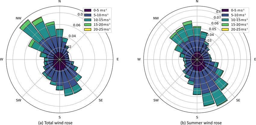
274                                           P. Fleming et al.: Initial results from a field campaign of wake steering – Part 1

Niayifar and Porté-Agel (2015). Annoni et al. (2018) pro-            The paper is organized as follows. Section 2 provides an
vide a detailed description of the current FLORIS model.           overview of the field campaign’s layout of turbines and sen-
The FLORIS model is open source and available for down-            sors, as well as meteorological conditions. Section 3 dis-
load and collaborative development (https://github.com/nrel/       cusses the implemented controller. Section 4 describes the
FLORIS, version 1.0.0, last access: 1 May 2019). Develop-          data collected in terms of total amount and characteristics.
ment is ongoing, and future models will incorporate the ad-        The performance of the controller, specifically in terms of
vances proposed in Martínez-Tossas et al. (2018).                  achieving targeted offsets, is reviewed in Sect. 5. Challenges
   Critical to advancement, improvement, and eventual adop-        specific to this first phase are described in Sect. 6. Finally,
tion of wake steering are field trials of wake steering in re-     Sect. 7 presents the results.
alistic environments. Wagenaar et al. (2012) attempted wake
steering at a scaled wind farm. One important campaign took
place at the National Wind Technology Center in Boulder,
Colorado. In that study, a rear-facing scanning lidar from the     2   Field campaign
University of Stuttgart was placed on top of the nacelle of
a GE 1.5 MW turbine, which held various yaw offset posi-           A subsection of a commercial wind farm was selected as the
tions for periods of 1 h at a time (Fleming et al., 2017a).        test site for the wake steering campaign. The site was cho-
The data from that campaign were used to investigate the           sen to include a set of turbines for which the main wind di-
accuracy of predictions made by FLORIS (Annoni et al.,             rections that generate strong waking conditions would occur
2018) and the impact on turbine loads caused by yaw offsets        relatively frequently and the turbines were close enough for
(Damiani et al., 2017). A related campaign is being under-         wake steering effects to be discernible. The selected wind
taken at the Scaled Wind Farm Technology facility in Lub-          farm subsection is shown in Fig. 1.
bock, Texas. Similar to the National Wind Technology Cen-             Five turbines (Fig. 1) are located in one corner of the farm.
ter study, a rear-facing lidar (in this case the Technical Uni-    Note that there are no turbines to the north or south, making
versity of Denmark spinner lidar) is used to scan the wake         these wind directions effectively free stream. The five tur-
of a V27 experimental turbine. The resulting data are used         bines are relatively closely spaced, especially the three tur-
to examine wake behavior (Herges et al., 2017) and under-          bines labeled T2, T3, and T4. T2 and T4 were controlled
stand loading impacts (White et al., 2018). Finally, a first       turbines, and T3 was selected as the downstream turbine to
published field trial at a commercial offshore wind farm is        be evaluated based on the wake impacts of T2 and T4. The
presented in Fleming et al. (2017b). In that study, a single       wind directions at which T2 (324◦ ) and T4 (134◦ ) directly
turbine implements a yaw offset control strategy to benefit        wake T3 are indicated in Fig. 1. T1 and T5 serve as reference
three downstream turbines.                                         turbines that are uncontrolled and unaffected by the control
   Still, there is a need for more conclusive field campaigns      turbines during wind conditions under which controls would
on the performance of wake steering and the evaluation of          be applied. Figure 2 illustrates the directional conventions for
the latest models. For this reason, a new field campaign was       steering applied to the T4 and T3 turbine pair.
initiated as a collaboration between the National Renewable           The terrain of the site is also illustrated in Fig. 1. Gen-
Energy Laboratory (NREL) and NextEra Energy Resources.             erally, the terrain to the north is flat, whereas the terrain to
A portion of a commercial wind farm was selected as a test         the south is complex (some escarpments can be seen in the
site, and significant additional sensing equipment is being        southwest in Fig. 1, and these extend to the south of T4).
deployed, including a (ground-based) lidar, meteorological         The campaign is divided into the “north” campaign, wherein
(met) tower, and two sodars. Additional nacelle-based lidars       flows from the north arrive over flat terrain and T2 is the
are being deployed for the upcoming second phase. Wake             controlled turbine, and the “south” campaign, wherein flows
steering controls based on the latest version of FLORIS are        from the south arrive over complex terrain and are expected
implemented on two turbines. This paper presents the results       to be more turbulent.
of the first phase of this campaign focused on wake steering.         The locations of the meteorological equipment are indi-
   The main contribution of this paper is the initial results      cated in Fig. 1. Based on the simpler terrain and overall wind
and analysis of a land-based wake steering field-test cam-         rose, the equipment is placed to prioritize the north cam-
paign. The paper presents the controller as implemented in         paign. A Leosphere Windcube v2 profiling lidar (shown in
the present phase and proposes improvements based on these         Fig. 1) provides profiles of wind speed and wind direction
initial results. The performance of wake steering, in terms of     calculated nominally every second but averaged to 1 min in-
increased energy production, is analyzed and compared with         tervals. This lidar (similar to that used in Lundquist et al.,
predictions from the FLORIS code. In addition, the wake            2017) samples line-of-sight velocities in four cardinal direc-
steering performance is assessed with respect to atmospheric       tions along a nominally 28◦ azimuth from vertical, followed
stability, which can be estimated using sensing available on       by a fifth vertically pointed beam. Range gates were centered
the met mast. Finally, several practical lessons learned are       every 20 m from 40 m up to 180 m. The sodars used in the
discussed.                                                         campaign are Vaisala Triton Wind Profilers. The sodars pro-

Wind Energ. Sci., 4, 273–285, 2019                                                        www.wind-energ-sci.net/4/273/2019/
P. Fleming et al.: Initial results from a field campaign of wake steering – Part 1                                                275

Figure 1. Layout of the experimental site. Turbine 2 (T2) and Turbine 4 (T4) have wake steering implemented to benefit Turbine 3 (T3),
whereas Turbine 1 (T1) and Turbine 5 (T5) are reference turbines. The position of the installed meteorological equipment is also shown.
Finally, the complexity of the terrain to the south and the flat terrain to the north are indicated.

                                                                      the months during which the campaign was run with more
                                                                      frequent south-southeasterly winds.
                                                                         Controllers were implemented and running on both T2 and
                                                                      T4. Because the south-southeasterly winds are more promi-
                                                                      nent in this season, phase 1 focuses on the south campaign as
                                                                      most of the collected data correspond to this direction. The
                                                                      final study will consider the north experiment as well. Be-
                                                                      cause of this focus on the south campaign, the most relevant
                                                                      components in Fig. 1 are T4 (controlled turbine), T3 (down-
                                                                      stream turbine), and the south sodar to measure inflow.

Figure 2. Illustration of wake steering showing that a positive yaw   3   Controller
offset is meant to indicate a counterclockwise rotation of the con-
trolled turbine.                                                      The controller implemented onto T4 was designed by opti-
                                                                      mizing a FLORIS model of the site based on wind direction
                                                                      and wind speed. This resulted in a lookup table, which pro-
vide measurements of wind speed and wind direction every              vides a desired yaw offset for T4 as a function of wind speed
20 m up to 200 m.                                                     and direction. Figure 4 shows this target offset function as a
   Phase 1 of the field campaign uses an initial deployment of        function of wind direction for several wind speeds. The ma-
the wake steering controller and initial collection of data over      genta lines indicate the approximate boundary of control and
the summer of 2018 (from 4 May through 11 July 2018). The             will be reused in upcoming figures to distinguish controlled
wind resource is seasonal: in the summer, southern winds              and uncontrolled wind directions. The offset is largest around
are more probable than northern winds. Figure 3 shows two             the peak wake loss direction near 134◦ and decreases as the
wind roses for the site, for which data were obtained us-             wind rotates southerly.
ing the NREL Wind Integration National Dataset tool kit                  These offset tables were constrained to be below the load
at 100 m of height. Figure 3a shows the annual wind rose,             impact limitations determined by Damiani et al. (2017). A
with winds coming dominantly from the north-northwest and             safe load envelope was determined to be yaw offset angles
south-southeast. Figure 3b shows the expected wind rose for           no larger than 20◦ during wind speeds of 12 m s−1 or less.

www.wind-energ-sci.net/4/273/2019/                                                            Wind Energ. Sci., 4, 273–285, 2019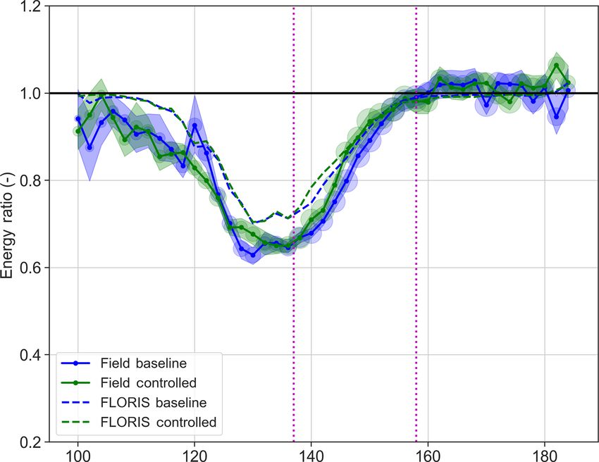
276                                                P. Fleming et al.: Initial results from a field campaign of wake steering – Part 1

Figure 3. Total wind rose for the site and for the particular months encompassing the test based on data collected from https://www.nrel.
gov/grid/wind-toolkit.html (last access: 1 May 2019).

                                                                            The controller in Fig. 5 computes a wind speed and wind
                                                                         direction from sensors available on each turbine. It then fil-
                                                                         ters both of these signals to remove high-frequency changes.
                                                                         The signals are fed into a lookup table, which is also filtered,
                                                                         and then the modified offset vane signal is sent to the turbine
                                                                         yaw controller.
                                                                            The offset function is toggled on and off every hour, as
                                                                         indicated in the diagram. This toggling enables the perfor-
                                                                         mance of the wake steering controller to be compared to a
                                                                         baseline control dataset that includes a similar composition
                                                                         of wind speeds. The decision to toggle every hour was a
                                                                         balance between accounting for the slowness of most yaw
                                                                         controllers and the variation of wind conditions. The optimal
                                                                         toggling period should be studied in more detail in the future
                                                                         to optimize the usefulness of the data collected.

Figure 4. Target offset for 8, 9, 10 and 11 m s−1 . The red line indi-
cates the target offset by wind direction. The magenta vertical lines    4   Data collection
indicate the approximate boundaries of the experiment (these vary
slightly by wind speed, but the overall shape is the same).              The phase 1 campaign lasted for approximately 3 months,
                                                                         during which the wake steering offset controller on T4 was
                                                                         toggled on and off hourly. This section describes the inflow
Finally, offsets were restricted to the counterclockwise di-             conditions during this period.
rection with respect to the wind (when viewed from above).                  The inflow conditions are described from the south so-
   The yaw controllers of the controlled turbines were then              dar data. Wind speed and wind direction are computed by
modified to implement this yaw offset strategy. Specifically,            a weighted average of the sodar measurements at heights
the nacelle vane signal fed into the controller was modified             that are within the rotor area of the turbine similar to the
by the specified yaw offset amount in the lookup table to in-            rotor-equivalent wind speed (Wagner et al., 2014). Turbu-
duce the yaw controller to track an offset. An external wake             lence intensity (TI) is estimated at hub height by the sodar
steering controller was implemented to determine the offset              as the 10 min standard deviation of the wind speed divided
to apply at a given moment. The specific setup is shown in               by the mean wind speed. Finally, stability is quantified via
Fig. 5.                                                                  the Obukhov lengths (Stull, 2012). For this case the Obukhov

Wind Energ. Sci., 4, 273–285, 2019                                                              www.wind-energ-sci.net/4/273/2019/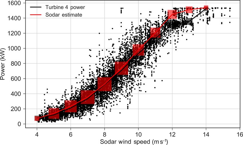
P. Fleming et al.: Initial results from a field campaign of wake steering – Part 1                                                          277

Figure 5. Block diagram of wake steering controller implementation. Inputs are provided by a typical turbine sensor, and the output is a
modified vane signal to supply the turbine yaw controller for wake steering. Note that this output is toggled on–off hourly. All low-pass filters
have a 30 s time constant.

Figure 6. Total data collection. The yellow bars indicate the data from unstable conditions, and the blue bars indicate the data from stable
conditions. The data were collected for both the baseline and controlled cases.

length L is computed via                                                      The total amount of data collected is summarized in Fig. 6.
                                                                           The amount of data collected between the “baseline” set, i.e.,
      −u3∗ θv                                                              controller off, and “controlled,” i.e., controller on, is com-
L=               ,                                                (1)
     Kgw 0 θv0                                                             parable. The data are broken into stable and unstable atmo-
                                                                           spheric conditions to show that toggling ensures that both
            2         2
                                                                           sets are similarly composed of atmospheric conditions.
u∗ = |u0 w0 + v 0 w 0 |1/4 ,                                      (2)         Atmospheric conditions are described in Fig. 7. In Fig. 7a,
                                                                           the wind directions observed over the course of the campaign
where K is the von Kármán constant assumed to be 0.4, u∗                   (as measured by the south sodar at hub height) are illustrated.
is the frictional velocity, g is gravity, θv is virtual potential          If data are restricted to points occurring in the range in which
temperature calculated with the met tower pressure at 2.5 m,               the experimental controller is active (in terms of wind speed
and u, v, and w are meteorological coordinates of wind                     and direction) and further limited by the removal of fault-
speed components in the west–east, south–north, and vertical               coded data or faulty sensing, the data are reduced to Fig. 7b.
planes; the 0 indicates perturbations. Fluxes were calculated              The distribution of wind speeds making up Fig. 7b are then
using a Reynolds decomposition based on a 30 min average.                  shown in Fig. 7c. Finally, Fig. 7d illustrates the recorded TI
Using the classification scheme of Wharton and Lundquist                   within the dataset remaining in Fig. 7b. The box sizes in
(2012), the data were divided into stable, neutral, and unsta-             Fig. 7d indicate the amount of data, and the data are subdi-
ble conditions. This division is simplified here so that “sta-             vided into stable and unstable categories to show that lower
ble” is defined as L < −1000 m and all other data are cate-                wind speeds are more likely to be higher-turbulence, unsta-
gorized as “not stable.”

www.wind-energ-sci.net/4/273/2019/                                                                   Wind Energ. Sci., 4, 273–285, 2019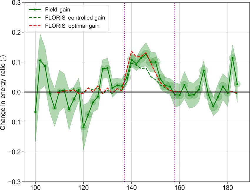
278 P. Fleming et al.: Initial results from a field campaign of wake steering – Part 1
Figure 7. Atmospheric conditions observed by the sodar at hub height over the duration of the test campaign.
ble conditions, whereas higher wind speeds tend to be low- most directions, except for a small band about the main wak-
turbulence stable conditions. The black line in Fig. 7d will ing direction. As the wind speed and direction drift in and
be used to describe the typical TI in the FLORIS model and out of controlled areas, the averaging effect biases the off-
will be discussed again later. set toward zero. This bias could be accounted for in future
controller design.
In addition to a steady bias toward smaller-than-targeted
5 Controller assessment
offsets, we also noticed a dynamic issue in the controller
design. The dynamic design of wind farm controllers is a
We first analyze the phase 1 data by considering the perfor-
field of active research (Bossanyi, 2018). In the initial design
mance of the controller in terms of its ability to produce a
phase, it was assumed that, to avoid excessive yawing be-
specific offset by wind speed and wind direction. The exact
haviors, we should low-pass filter the wind speed and wind
function of the turbine yaw controller is not known. There-
direction inputs to the lookup table, as well as the resultant
fore, it was difficult to know in advance how effective the
offset sent to the yaw controller. We did not account for the
method shown in Fig. 5 would be in delivering the desired
fact that the yaw controller itself acts as a lag filter between
offsets.
changes in wind direction and changes in nacelle yaw posi-
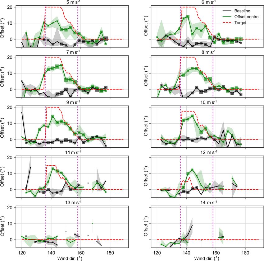
Figure 8 assesses the performance of this offset controller.
tion, so the yaw offset control system as a whole is prob-
Binned by wind speed, the figure shows the median main-
ably too slow and a general tendency toward overlagging
tained offset. The offset here is computed by comparing the
changes in wind direction was observed. This is illustrated
nacelle position of T4 with the measurement of wind direc-
in Fig. 9. At approximately 2 min, the wind direction crosses
tion recorded by the south sodar. Generally, the offsets are
into the region in which a 20◦ offset would be dictated by the
achieved reasonably well; however, there is a tendency to-
static optimal lookup table. The low-pass filtering, however,
ward undershoot. The undershoot could be an artifact of tem-
causes the offset target to lag until the third minute to reach
poral averaging over periods with and without offset, which
20◦ . Then, the filtering of the offset achieves 20◦ around the
biases computed offsets toward zero. However, we suspect
fourth minute. Further, the turbine is observed to begin yaw-
that the undershoot is actually occurring because of the fact
ing around the fourth minute and completes this action in the
that the actual controller is tracking an offset that is zero for
Wind Energ. Sci., 4, 273–285, 2019 www.wind-energ-sci.net/4/273/2019/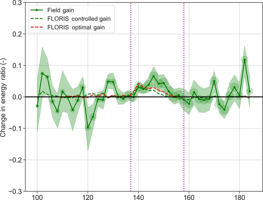
P. Fleming et al.: Initial results from a field campaign of wake steering – Part 1                                                   279

Figure 8. Comparison of observed yaw offset (green line) versus target (dashed red line) segregated by wind speeds. Note that the achieved
offset is computed as the difference between the sodar-measured wind direction and the turbine nacelle heading. Points indicate median
offset, with box size indicating the number of points in a bin and bands indicating the 95 % confidence interval of the median.

fifth minute, 3 min after the offset could have been optimally         but the version of FLORIS used in the design and analysis
applied. Some lag is unavoidable and potentially desirable to          has no terrain-modeling capabilities. This mismatch between
avoid adding too much additional yaw activity to the turbine,          the modeling assumptions and reality introduces a degree of
but based on this result, the controllers used in the upcoming         uncertainty. Second, T4 and T3 are spaced such that T3 is
phase 2 will be designed dynamically and the filter constants          in the near-wake region of T4. The version of FLORIS used
adjusted to account for this.                                          does not contain a well-tuned near-wake model. Finally, as
                                                                       shown in Fig. 6, the collected data are only about one-third
                                                                       composed of stable atmospheric conditions because of the
6   Challenges in this campaign                                        summer season and longer days. Stable, low-turbulence con-
                                                                       ditions would be more favorable to wake steering and may
This phase 1 campaign revealed several challenges that could           occur more frequently in the winter season.
inform future campaigns, including our future phases. De-                 A second set of challenges arises from more practical con-
spite these challenges, the wake steering controller did pro-          siderations. Specifically, the only sensor that could be used
duce the desired result of increasing power at the downstream          for the south experiment to measure the inflow is the south
turbine.                                                               sodar, as it is the only one to the south of T4. The south so-
   A first set of challenges corresponds to the site condi-            dar, in comparison to other instruments, was shown to mea-
tions for the south campaign. The topography is complex,

www.wind-energ-sci.net/4/273/2019/                                                              Wind Energ. Sci., 4, 273–285, 2019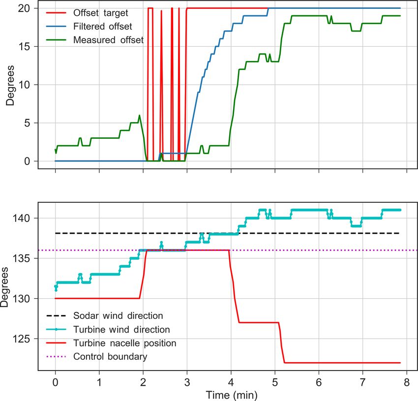
280                                              P. Fleming et al.: Initial results from a field campaign of wake steering – Part 1

                                                                      Figure 10. Sodar available power fit. The data from T4 are shown
                                                                      in black and the sodar estimate is shown in red. The red boxes refer
                                                                      to the wind speed bins and the size refers to the amount of data in
                                                                      each bin.

                                                                      allel to the upstream turbine on a line perpendicular to the
                                                                      controlled wind directions. In addition, the complex terrain
Figure 9. Time series data of T4 operation showing the sources of     varies from T1 to T5.
lag in yaw offset control. The figure shows that following the wind      For this reason, a synthetic reference turbine power was
direction entering the range at which a 20◦ offset would be optimal   used based on the measurements of the south sodar. The wind
at the 2 min mark, the offset is not actually achieved until 3 min    speeds at heights corresponding to the turbine rotor were
later.                                                                collected and applied to a weighted average, called Usodar ,
                                                                      wherein the weights were proportional to the sector of rotor
                                                                      area the heights correspond with, similar to a rotor-effective
sure the inflow well; however, it delivers data only once every
                                                                      wind speed calculation (Wagner et al., 2014). The hypotheti-
10 min, and this frequency is too coarse for the data analysis
                                                                      cal power of a reference turbine could then be computed us-
because 10 min will include a diverse mix of wind directions
                                                                      ing
and offsets. The turbine data are delivered at a frequency of
1 Hz, and through trial and error, a compromise of down-                                3
                                                                      Psodar = 0.5ρACp Usodar ,                                       (3)
sampling the turbine data to 1 min periods while up-sampling
the sodar data was selected (this up-sampling is done through         where Cp is derived from the Cp lookup table included in
a “zero-order hold”, wherein the data for each minute bin             FLORIS, ρ is the average observed density, and A is the rotor
are assigned the 10 min average). However, in the upcoming            area. This estimated sodar power was then compared with the
north campaign, more frequent data are available from the             measured power of T4 when the turbine is not intentionally
lidar and can be used.                                                operating in the offset condition (Fig. 10). The plot shows
   Finally, the controller design, wherein we influence the           that correspondence is very close except for near rated.
yaw controller without fully understanding its behavior, is              To analyze the effect of the wake steering implementation
a major challenge. If the yaw controller could be directly            on the control and downstream turbine, the following method
modified, the delays shown in Fig. 9 could be reduced and             of analysis is used. First, the data are limited to include only
performance improved.                                                 periods in which both turbines were operating normally and
                                                                      the quality of the sodar estimate was above a certain thresh-
7   Results                                                           old according to quality flags reported by the sodar at each
                                                                      range. Next, all the data, including the power of T3 and the
The first step in performing the analysis was selecting a ref-        sodar reference power, are binned into wind direction bins
erence for comparing the power of T3 and T4. In previous              every 2◦ (with 1◦ of overlap between adjacent bins as this
work, e.g., Fleming et al. (2017b), a reference uncontrolled          was found useful in clarifying trends in the available data)
turbine was preferred as it would provide a reference power           and according to whether the wake steering controller was
that includes the effects not only of wind speed, but also            toggled on (controlled) or off (baseline).
shear, veer, and TI. For this reason, both T1 and T5 were                Then for each bin, an energy ratio is computed, which in-
considered, but a significant amount of noise and noncor-             volves a weighted summation of all the power measurements
relation was observed, likely because both turbines are far           P Test of the test turbine (the determination of the weights w
downstream from T4. Ideally, the reference would be par-              will be detailed later), i.e., T3, and the reference turbine, i.e.,

Wind Energ. Sci., 4, 273–285, 2019                                                            www.wind-energ-sci.net/4/273/2019/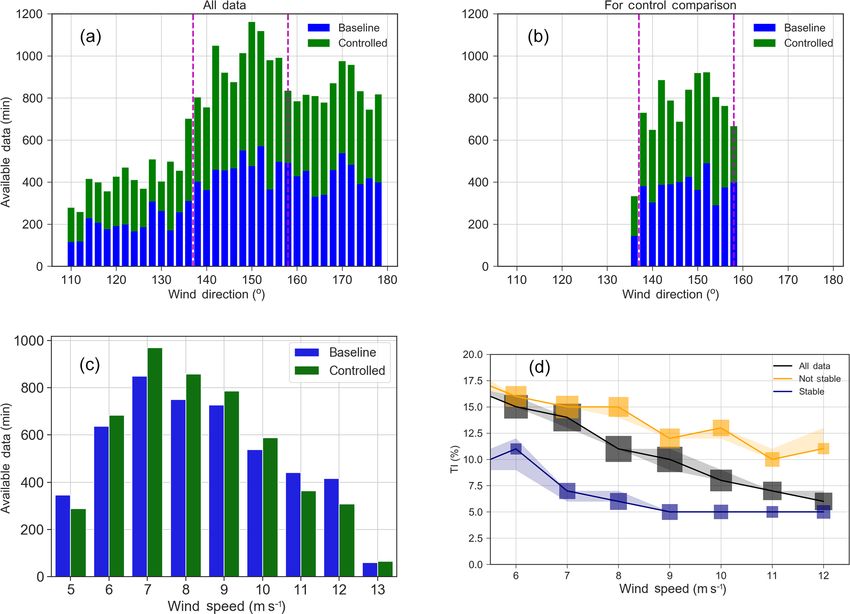
P. Fleming et al.: Initial results from a field campaign of wake steering – Part 1 281
sodar estimate P Ref , and then a ratio of the two. In addition to computing a single energy ratio for each bin,
PN the process is bootstrapped, whereby the data are randomly
wi PiTest sampled with replacement and the energy ratio recomputed
REnergy = Pi=1
N
(4)
Ref
i=1 wi Pi 1000 times or more depending on the amount of data. The
results of these bootstrap iterations are then used to compute
Note that this method is different from a power ratio
95 % confidence intervals, and these are indicated in the plots
method in which a power ratio is computed for each set of
of the energy ratio as semi-transparent bands.
points and then averaged.
The method of computing energy ratios is now in-
cluded within the open-source FLORIS model (https://floris.
!
N
1 X PiTest
RPower = (5) readthedocs.io, last access: 1 May 2019).
N i=1 PiRef
Note that all wind speeds are used in this calculation, in-
It is also different from the slope method used in Fleming cluding those (greater than 12 m s−1 ) in which the 0◦ offset
et al. (2017b). is actually targeted, even in the controller on mode. With the
10 min sodar rate and the lag of the controller, it is difficult to
draw an exact line where the controller stops impacting the
RSlope : min ||P Test − RSlope P Ref ||2 , (6) individual turbine yaw controller. Including all wind speeds
RSlope
also corresponds to the final change in energy.
where R[...] is the ratio computed through the different meth- The energy ratio calculation is repeated on several differ-
ods, P Test and P Ref are vectors of all observed powers for the ently defined FLORIS models of the site to provide a point
reference and test turbines, PiRef is a single-minute average, of comparison. An “aligned” case simulates every observed
and N is the total number of points in a given wind direction wind speed and direction in the baseline field data with all
bin. turbines perfectly aligned to the flow, while a baseline case
The energy ratio (Eq. 4) is used for a few reasons. First, uses the actual small offsets observed. An “optimal” case
changes in relative energy production are more directly re- simulates all the wind speeds and directions in the controlled
lated to changes in revenue. Second, the power ratio is an field data using the exact offset requested by the control strat-
average of ratios instead of the ratio of averages proposed in egy, while the controlled case applies the actual achieved off-
the energy ratio (Eq. 5). The power ratio is more sensitive to set. These four settings are summarized in Table 1. For each
small changes in power at low wind speeds that do not con- of the FLORIS models and for each 1 min wind speed and di-
tribute meaningfully to changes in energy production, which rection observed in the field, a matching FLORIS simulation
is the ultimate goal. The slope method (Eq. 6) of Fleming was run, the power of T3 and T4 tabulated, and the energy
et al. (2017b) was able to achieve a weighting of higher wind ratio computed. When considering gains in energy, FLORIS
speeds through slope fitting. However, the energy ratio was optimal gain refers to the change from aligned to optimal,
finally thought to be more directly related to annual energy whereas FLORIS controlled gain refers to the change from
production, the overall quantity of interest. The energy ratio baseline to controlled.
represents the increase or decrease in energy produced for a The energy ratios can be computed from these FLORIS
specific wind direction bin. models. The comparison of the aligned and optimal case
In computing the energy ratio, a wind-speed-based weight- should present an upper bound on performance if exact off-
ing strategy helps to more quickly converge the analysis and sets and alignments held, whereas the baseline and controlled
reduce changes in energy ratios due to variations in the com- cases show what we expect from this dataset.
positions of wind speeds for the two controllers within each
wind direction bin with respect to differences due to changes 7.1 Turbine 3 analysis
in controller. The main idea is that for each wind direction,
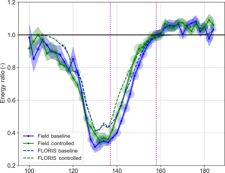
the power values collected are binned according to wind Figure 11 shows the energy ratios by wind direction for T3.
speed (as measured by the sodar) and the total energy for The wake loss is deeper than FLORIS expects (T3 is produc-
the baseline and controlled cases is the weighted sum of the ing less than 40 % of the energy of the reference at nadir);
powers; the weight is the number of points the other control however, as mentioned, this is a difficulty of current near-
setting has in this wind speed bin out of the total. For ex- wake models and the subject of active research. Still, the gain
ample, if there are 10 samples of baseline taken at 13 m s−1 in energy production in the wind direction for which the con-
and 5 of controlled, the baseline points are weighted by 1/3 troller is active is observed. Note that as described earlier, to
and the controlled by 2/3, so the final energy ratios to be clarify trends, the wind direction bins are every 2◦ but are 3◦
compared are more approximately even in terms of the wind wide (overlapping with adjacent) to increase the number of
speed distributions represented. If the bins are perfectly bal- points available per bin.
anced, there are an equivalent number of baseline and con- The difference between the baseline and controlled cases
trolled points at each wind speed, and the weights have no for both the field data and FLORIS quantifies the impact of
effect. yaw control on power production (Fig. 12). In the 10◦ sector
www.wind-energ-sci.net/4/273/2019/ Wind Energ. Sci., 4, 273–285, 2019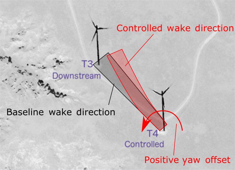
282                                               P. Fleming et al.: Initial results from a field campaign of wake steering – Part 1

Table 1. FLORIS model definitions for comparison. The columns yaw 4 and yaw 3 determine what sets the yaw angle for each turbine
(aligned is always 0◦ ), with optimal being the true optimal; “from baseline” means applying the observed yaw angles from the baseline data
of the field campaign. Wind conditions are similarly defined.

                                 Model          Yaw 4               Yaw 3             Wind conditions
                                 Aligned        Aligned             Aligned           From baseline data
                                 Baseline       From baseline       From baseline     From baseline data
                                 Optimal        Optimal             Aligned           From controlled data
                                 Controlled     From controlled     From controlled   From controlled data

Figure 11. Energy ratio for T3 for field data and the baseline and       Figure 12. Change in the energy ratio of T3 from field data. Expec-
controlled FLORIS cases (see Table 1). An energy ratio of 0.5 cor-       tations from FLORIS using the actually achieved controlled offsets
responds to a production of 50 % of the total expected based on the      (controlled − baseline) and optimal (optimal − aligned) are shown
measured inflow without considering wakes. The vertical magenta          to indicate comparison with expectations given control values and
lines indicate the region where control is applied and a difference      what is optimally expected.
between the baseline and controlled is expected. The size of the cir-
cles at each point indicates the number of points in the bin, while
the bands indicate 95 % confidence as computed by bootstrapping.         7.2    Aggregate analysis

                                                                         Finally, the previously mentioned analysis is repeated, but
between 140 and 150◦ the average gain in energy is 14.6 %.               using the aggregated power of T4 and T3, so that the losses
Compared to FLORIS predictions, the field results compare                in energy coming from offsetting the yaw of T4 are deducted
favorably to the estimations from FLORIS. The data outside               from the gains made downstream (Fig. 14 shows the energy
of the control bands, while noisy, indicate an average around            ratios and Fig. 15 shows the difference between them). The
0, underlining the significance of the nonzero apparent aver-            aggregated energy gains appear to be somewhat more than
age in the control region.                                               the current version of FLORIS expects (a net gain of 4.1 %
   Figure 13 segregates stable conditions from unstable con-             over the same 10◦ region from 140 to 150◦ ), but this could
ditions and repeats the analysis of Figs. 11 and 12. The gain            again be connected to difficulty measuring the near wake.
in stable conditions is more consistently realized (as indi-
cated by the bands) and the peak gain is higher than in un-
                                                                         8     Conclusions
stable conditions. This distinct improvement in stable con-
ditions could be because wake steering is more effective in              We present the initial results from the first phase of a field
stable conditions. Additionally, in stable conditions, atmo-             campaign evaluating wake steering at a commercial wind
spheric inflow is more homogeneous and therefore easier to               farm. For two closely spaced turbines, an approximate 14 %
measure. Upcoming winter measurements from the north for                 increase in energy was measured on the downstream turbine
phase 2 will consist of more stable measurements due to the              over a 10◦ sector with a 4 % increase in energy when ac-
longer nights and may shed more light on the role of atmo-               counting for losses of the upstream turbine. The gains in en-
spheric stability in wake steering.                                      ergy were compared to predictions made using the FLORIS

Wind Energ. Sci., 4, 273–285, 2019                                                               www.wind-energ-sci.net/4/273/2019/
P. Fleming et al.: Initial results from a field campaign of wake steering – Part 1 283 Figure 13. Energy ratio of T3, as in Fig. 11, divided into stable and unstable conditions. Figure 14. Energy ratio of the summed energy of T3 and T4. Figure 15. Combined change in energy ratio for T3 and T4. model used to design the applied controllers. The overall accurately modeling the wake losses and therefore may have gains were consistent with predictions from FLORIS. realized a less-than-optimal controller. Still, the overall gains This initial stage of the wake steering campaign identified in energy were in line with prior expectations from FLORIS. several areas for improvement in future work, such as aspects All together, the authors hope that the results presented of dynamic controller design, time filtering, and uncertainty might therefore represent a baseline for the possibility of quantification. Difficulties with this particular south cam- gains from wake steering. Better modeling and controls, sim- paign, including complex terrain and summer atmospheric pler site conditions, and the exploitation of vortex modeling conditions, were identified as possible sources of improve- and larger arrays of turbines all present hopeful avenues for ment as the campaign moves to northern winter conditions. continued improvements. An upcoming companion paper on Additionally, near-wake modeling presented a challenge in the second phase of the experiment will review results, in- www.wind-energ-sci.net/4/273/2019/ Wind Energ. Sci., 4, 273–285, 2019
284                                               P. Fleming et al.: Initial results from a field campaign of wake steering – Part 1

cluding the opportunities for improvement identified in this            Damiani, R., Dana, S., Annoni, J., Fleming, P., Roadman, J., van
paper.                                                                     Dam, J., and Dykes, K.: Assessment of wind turbine component
                                                                           loads under yaw-offset conditions, Wind Energ. Sci., 3, 173–189,
                                                                           https://doi.org/10.5194/wes-3-173-2018, 2018.
Data availability. Currently, the data are not publicly available;      Fleming, P., Gebraad, P. M., Lee, S., Wingerden, J.-W., Johnson,
however, if in the future portions of the data become available, this      K., Churchfield, M., Michalakes, J., Spalart, P., and Moriarty, P.:
would be through the DOE A2e data portal at https://a2e.energy.            Simulation comparison of wake mitigation control strategies for
gov/about/dap.                                                             a two-turbine case, Wind Energy, 18, 2135–2143, 2015.
                                                                        Fleming, P., Annoni, J., Scholbrock, A., Quon, E., Dana, S.,
                                                                           Schreck, S., Raach, S., Haizmann, F., and Schlipf, D.: Full-scale
                                                                           field test of wake steering, J. Phys. Conf. Ser., 854, 012013,
Author contributions. All coauthors were involved in writing
                                                                           https://doi.org/10.1088/1742-6596/854/1/012013, 2017a.
and editing the paper. The design of the controller and analysis of
                                                                        Fleming, P., Annoni, J., Shah, J. J., Wang, L., Ananthan, S., Zhang,
data were performed by PF, JK, KD, ES, PM, JKL, KF, CB, RM,
                                                                           Z., Hutchings, K., Wang, P., Chen, W., and Chen, L.: Field test
and PM. The implementation of experiments at the site was done by
                                                                           of wake steering at an offshore wind farm, Wind Energ. Sci., 2,
JR, AS, JvD, HL, JS, MS, BR, CG, and DB.
                                                                           229-239, https://doi.org/10.5194/wes-2-229-2017, 2017b.
                                                                        Gebraad, P., Teeuwisse, F., Wingerden, J., Fleming, P. A., Ruben, S.,
                                                                           Marden, J., and Pao, L.: Wind plant power optimization through
Competing interests. The authors declare that they have no con-            yaw control using a parametric model for wake effects – a CFD
flict of interest.                                                         simulation study, Wind Energy, 19, 95–114, 2016.
                                                                        Herges, T., Maniaci, D. C., Naughton, B. T., Mikkelsen, T., and
                                                                           Sjöholm, M.: High resolution wind turbine wake measure-
Disclaimer. The views expressed in the article do not necessarily          ments with a scanning lidar, J. Phys. Conf. Ser., 854, 012021,
represent the views of the DOE or the U.S. Government.                     https://doi.org/10.1088/1742-6596/854/1/012021, 2017.
                                                                        Howland, M. F., Bossuyt, J., Martinez-Tossas, L. A., Meyers, J., and
                                                                           Meneveau, C.: Wake structure in actuator disk models of wind
Financial support. Funding provided by the U.S. Department of              turbines in yaw under uniform inflow conditions, J. Renew. Sus-
Energy Office of Energy Efficiency and Renewable Energy Wind               tain. Energ., 8, 043301, https://doi.org/10.1063/1.4955091, 2016.
Energy Technologies Office.                                             Jensen, N. O.: A note on wind generator interaction, Tech. Rep.
                                                                           Risø-M-2411, Risø National Laboratory, 1984.
                                                                        Jiménez, Á., Crespo, A., and Migoya, E.: Application of a LES tech-
Review statement. This paper was edited by Sandrine Aubrun                 nique to characterize the wake deflection of a wind turbine in
and reviewed by two anonymous referees.                                    yaw, Wind Energy, 13, 559–572, 2010.
                                                                        Lundquist, J. K., Wilczak, J. M., Ashton, R., Bianco, L., Brewer,
                                                                           W. A., Choukulkar, A., Clifton, A., Debnath, M., Delgado, R.,
                                                                           Friedrich, K., Gunter, S., Hamidi, A., Iungo, G. V., Kaushik,
                                                                           A., Kosović, B., Langan, P., Lass, A., Lavin, E., Lee, J. C.-Y.,
References                                                                 McCaffrey, K. L., Newsom, R. K., Noone, D. C., Oncley, S. P.,
                                                                           Quelet, P. T., Sandberg, S. P., Schroeder, J. L., Shaw, W. J., Spar-
Annoni, J., Fleming, P., Scholbrock, A., Roadman, J., Dana,                ling, L., Martin, C. S., Pe, A. S., Strobach, E., Tay, K., Van-
  S., Adcock, C., Porte-Agel, F., Raach, S., Haizmann, F.,                 derwende, B. J., Weickmann, A., Wolfe, D., and Worsnop, R.:
  and Schlipf, D.: Analysis of control-oriented wake modeling              Assessing State-of-the-Art Capabilities for Probing the Atmo-
  tools using lidar field results, Wind Energ. Sci., 3, 819–831,           spheric Boundary Layer: The XPIA Field Campaign, B. Am.
  https://doi.org/10.5194/wes-3-819-2018, 2018.                            Meteorol. Soc., 98, 289–314, https://doi.org/10.1175/BAMS-D-
Bartl, J., Mühle, F., and Sætran, L.: Wind tunnel study on                 15-00151.1, 2017.
  power output and yaw moments for two yaw-controlled                   Martínez-Tossas, L. A., Annoni, J., Fleming, P. A., and Church-
  model wind turbines, Wind Energ. Sci., 3, 489–502,                       field, M. J.: The aerodynamics of the curled wake: a simplified
  https://doi.org/10.5194/wes-3-489-2018, 2018.                            model in view of flow control, Wind Energ. Sci., 4, 127–138,
Bastankhah, M. and Porté-Agel, F.: A new analytical model for              https://doi.org/10.5194/wes-4-127-2019, 2019.
  wind-turbine wakes, Renew. Energ., 70, 116–123, 2014.                 Medici, D. and Alfredsson, P.: Measurements on a wind turbine
Bastankhah, M. and Porté-Agel, F.: Experimental and theoretical            wake: 3D effects and bluff body vortex shedding, Wind Energy,
  study of wind turbine wakes in yawed conditions, J. Fluid Mech.,         9, 219–236, 2006.
  806, 506–541, 2016.                                                   Niayifar, A. and Porté-Agel, F.: A new analytical model for
Bossanyi, E.: Combining induction control and wake steer-                  wind farm power prediction, J. Phys. Conf. Ser., 625, 012039,
  ing for wind farm energy and fatigue loads optimisation, J.              https://doi.org/10.1088/1742-6596/625/1/012039, 2015.
  Phys. Conf. Ser., 1037, 032011, https://doi.org/10.1088/1742-         NREL: FLORIS, Version 1.0.0, available at: https://github.com/
  6596/1037/3/032011, 2018.                                                NREL/floris, last access: 1 May 2019.
Dahlberg, J. and Medici, D.: Potential improvement of wind turbine
  array efficiency by active wake control (AWC), in: Proc Euro-
  pean Wind Energy Conference, 65–84, 2003.

Wind Energ. Sci., 4, 273–285, 2019                                                                www.wind-energ-sci.net/4/273/2019/
P. Fleming et al.: Initial results from a field campaign of wake steering – Part 1 285 Park, J., Kwon, S.-D., and Law, K. H.: A data-driven approach for Wagner, R., Cañadillas, B., Clifton, A., Feeney, S., Ny- cooperative wind farm control, in: American Control Conference gaard, N., Poodt, M., St Martin, C., Tüxen, E., and Wa- (ACC), IEEE 2016, 525–530, 2016. genaar, J.: Rotor equivalent wind speed for power curve Schottler, J., Mühle, F., Bartl, J., Peinke, J., Adaramola, M. S., Sæ- measurement–comparative exercise for IEA Wind Annex 32, tran, L., and Hölling, M.: Comparative study on the wake deflec- J. Phys. Conf. Ser., 524, 012108, https://doi.org/10.1088/1742- tion behind yawed wind turbine models, J. Phys. Conf. Ser., 854, 6596/524/1/012108, 2014. 012032, https://doi.org/10.1088/1742-6596/854/1/012032, 2017. Wharton, S. and Lundquist, J. K.: Atmospheric stability affects Stull, R. B.: An introduction to boundary layer meteorology, vol. 13, wind turbine power collection, Environ. Res. Lett., 7, 014005, Springer Science & Business Media, 2012. https://doi.org/10.1088/1748-9326/7/1/014005, 2012. Vollmer, L., Steinfeld, G., Heinemann, D., and Kühn, M.: Estimat- White, J., Ennis, B., and Herges, T. G.: Estimation of Ro- ing the wake deflection downstream of a wind turbine in different tor Loads Due to Wake Steering, in: 2018 Wind En- atmospheric stabilities: an LES study, Wind Energ. Sci., 1, 129– ergy Symposium, Kissimmee, Florida, 8–12 January 2018, 141, https://doi.org/10.5194/wes-1-129-2016, 2016. https://doi.org/10.2514/6.2018-1730, 2018. Wagenaar, J., Machielse, L., and Schepers, J.: Controlling wind in ECN’s scaled wind farm, Proc. Europe Premier Wind Energy Event, Copenhage, Denmark, 16–19 April 2012, ECN, 685–694, 2012. www.wind-energ-sci.net/4/273/2019/ Wind Energ. Sci., 4, 273–285, 2019
You can also read