ISOMETRIC PROPAGATION NETWORK FOR GENERALIZED ZERO-SHOT LEARNING - OpenReview
←
→
Page content transcription
If your browser does not render page correctly, please read the page content below
Published as a conference paper at ICLR 2021

I SOMETRIC P ROPAGATION N ETWORK
FOR G ENERALIZED Z ERO - SHOT L EARNING

  Lu Liu† , Tianyi Zhou‡ , Guodong Long† , Jing Jiang† , Xuanyi Dong† , Chengqi Zhang†
 † University of Technology Sydney, ‡ University of Washington
 Corresponding to: lu.liu.cs@icloud.com

                                            A BSTRACT

         Zero-shot learning (ZSL) aims to classify images of an unseen class only based on
         a few attributes describing that class but no access to any training sample. A pop-
         ular strategy is to learn a mapping between the semantic space of class attributes
         and the visual space of images based on the seen classes and their data. Thus,
         an unseen class image can be ideally mapped to its corresponding class attributes.
         The key challenge is how to align the representations in the two spaces. For most
         ZSL settings, the attributes for each seen/unseen class are only represented by a
         vector while the seen-class data provide much more information. Thus, the im-
         balanced supervision from the semantic and the visual space can make the learned
         mapping easily overfitting to the seen classes. To resolve this problem, we pro-
         pose Isometric Propagation Network (IPN), which learns to strengthen the re-
         lation between classes within each space and align the class dependency in the
         two spaces. Specifically, IPN learns to propagate the class representations on an
         auto-generated graph within each space. In contrast to only aligning the resulted
         static representation, we regularize the two dynamic propagation procedures to
         be isometric in terms of the two graphs’ edge weights per step by minimizing
         a consistency loss between them. IPN achieves state-of-the-art performance on
         three popular ZSL benchmarks. To evaluate the generalization capability of IPN,
         we further build two larger benchmarks with more diverse unseen classes, and
         demonstrate the advantages of IPN on them.

1   I NTRODUCTION

One primary challenge on the track from artificial intelligence to human-level intelligence is to
improve the generalization capability of machine learning models to unseen problems. While most
supervised learning methods focus on generalization to unseen data from training task/classes, zero-
shot learning (ZSL) (Larochelle et al., 2008; Lampert et al., 2014; Xian et al., 2019a) has a more
ambitious goal targeting the generalization to new tasks and unseen classes. In the context of image
classification, given images from some training classes, ZSL aims to classify new images from
unseen classes with zero training image available. Without training data, it is impossible to directly
learn a mapping from the input space to the unseen classes. Hence, recent works introduced learning
to map between the semantic space and visual space (Zhu et al., 2019a; Li et al., 2017; Jiang et al.,
2018) so that the query image representation and the class representation can be mapped to a shared
space for comparison.
However, learning to align the representation usually leads to overfitting on seen classes (Liu et al.,
2018). One of the reasons is that in most zero-shot learning settings, the number of images per class
is hundreds while the semantic information provided for one class is only limited to one vector.
Thus, the mapping function is easily overfitting to the seen classes when trained using the small set
of attributes. The learned model typically has imbalanced performance on samples from the seen
classes and unseen classes, i.e., strong when predicting samples from the seen classes but struggles
in the prediction for samples in the unseen classes.
In this paper, we propose “Isometric Propagation Network (IPN)” which learns to dynamically
interact between the visual space and the semantic space. Within each space, IPN uses an attention
module to generate a category graph, and then perform multiple steps of propagation on the graph.

                                                  1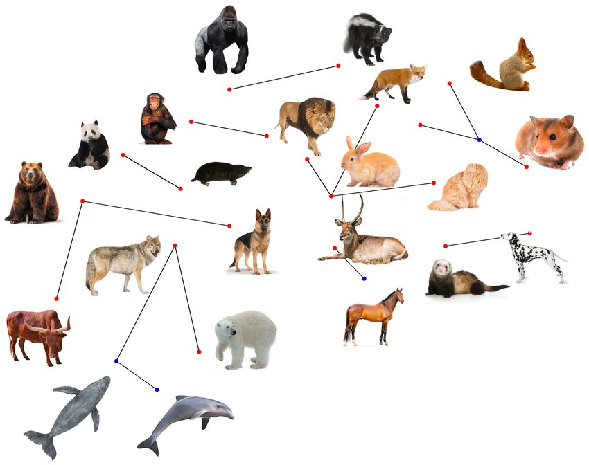
Published as a conference paper at ICLR 2021

    (a) visual class prototypes       (b) semantic class prototypes
                                                                           (c) concatenated dual prototypes
      and the generated graph            and the generated graph

Figure 1: t-SNE (Maaten & Hinton, 2008) of the prototypes produced by IPN on AWA2. Blue/red
points represent unseen/seen classes.

In every step, the distribution of the attention scores generated in each space are regularized to be
isometric so that implicitly aligns the relationships between classes in two spaces. Due to different
motifs of the generated graphs, the regularizer for the isometry between the two distributions are
provided with sufficient training supervisions and can potentially generalize better on unseen classes.
To get more diverse graph motifs, we also apply episodic training which samples different subset of
classes as the nodes for every training episode rather than the whole set of seen classes all the time.
To evaluate IPN, we compared it with several state-of-the-art ZSL methods on three popular ZSL
benchmarks, i.e., AWA2 (Xian et al., 2019a), CUB (Welinder et al., 2010) and aPY (Farhadi et al.,
2009). To test the generalization ability on more diverse unseen classes rather than similar classes to
the seen classes, e.g., all animals for AWA2 and all birds for CUB, we also evaluate IPN on two new
large-scale datasets extracted from tieredImageNet (Ren et al., 2018), i.e., tieredImageNet-Mixed
and tieredImageNet-Segregated. IPN consistently achieves state-of-the-art performance in terms of
the harmonic mean of the accuracy on unseen and seen classes. We show the ablation study of each
component in our model and visualize the final learned representation in each space in Figure 1. It
shows the class representations in each space learned by IPN are evenly distributed and connected
smoothly between the seen and unseen classes. The two spaces can also reflect each other.

2    R ELATED W ORKS
Most ZSL methods can be categorized as either discriminative or generative. Discriminative meth-
ods generate the classifiers for unseen classes from its attributes by learning a mapping from a input
image’s visual features to the associated class’s attributes on training data of seen classes (Frome
et al., 2013; Akata et al., 2015a;b; Romera-Paredes & Torr, 2015; Kodirov et al., 2017; Socher
et al., 2013; Cacheux et al., 2019; Li et al., 2019b), or by relating similar classes according to
their shared properties, e.g., semantic features (Norouzi et al., 2013; Chi et al., 2021) or phantom
classes (Changpinyo et al., 2016), etc. In contrast, generative methods employ the recently popular
image generation models (Goodfellow et al., 2014) to synthesize images of unseen classes, which
reduces ZSL to supervised learning (Huang et al., 2019) but usually increases the training cost and
model complexity. In addition, the study of unsupervised learning (Fan et al., 2021; Liu et al., 2021),
meta learning (Santoro et al., 2016; Liu et al., 2019b;a; Ding et al., 2020; 2021), or architecture de-
sign (Dong et al., 2021; Dong & Yang, 2019) can also be used improve the representation ability of
visual or semantic features.
Alignment between two spaces in ZSL Frome et al. (2013); Socher et al. (2013); Zhang et al.
(2017) proposed to transform representations either to the visual space or the semantic space for
distance for comparison. Li et al. (2017) introduces how to optimize the semantic space so that
the two spaces can be better aligned. Jiang et al. (2018); Liu et al. (2020) tries to map the class
representations from two spaces to another common space. Comparatively, our IPN does not align
two spaces by feature transformation but by regularizing the isometry of the intermediate output
from two propagation model.
Graph in ZSL Graph structures have already been explored for their benefits to some discriminative
ZSL models, e.g., Wang et al. (2018); Kampffmeyer et al. (2019) learn to generate the weights of
a fully-connected classifier for a given class based on its semantic features computed on a pre-

                                                         2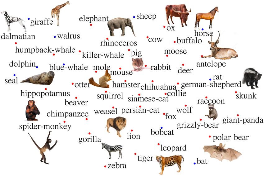
Published as a conference paper at ICLR 2021

Figure 2: LEFT: The pipeline of IPN. First, we initialize the visual and semantic prototypes from
seen classes’s data and class attributes. Then, prototype propagation in each space can be per-
formed over multiple steps. Finally, the concatenated prototypes form the support set of a distance
based classifier. RIGHT: Isometric propagation. we propagate prototypes of each class to other
connected classes on the graph using attention module. The attention score is regularized to be
isometric.

defined semantic graph using a graph convolutional networks (GCN). They require (1) a pre-trained
CNN whose last fully-connected layer provides the ground truth of the classifiers ZSL aims to
generate; and (2) an existing knowledge graph as the input of GCN. By contrast, our method learns
to automatically generate the graph and the class prototypes composing the support set of a distance-
based classifier. Hence, our method does not require a pre-trained CNN to provide a ground truth
for the classifier. In addition, we train a modified graph attention network (GAN) (rather than a
GCN) to generate the prototypes, so it learns both the class adjacency and edges by itself and can
provide more accurate modeling of class dependency in scenarios when no knowledge graph is
provided. Tong et al. (2019) and Xie et al. (2020) also leverage the idea of graph to transform the
feature extracted from the CNN while our graph serves as the paths for propagation. It requires
an off-the-shelf graph generated by ConceptNet (Speer et al., 2016), while IPN applies prototype
propagation and learns to construct the graph in an end-to-end manner.
Attention in ZSL The attention module has been applied for zero-shot learning for localization.
Liu et al. (2019c) introduces localization on the semantic information and Xie et al. (2019) proposes
localization on the visual feature. Zhu et al. (2019b) further extends it to multi-localization guided
by semantic. Different from them, our attention serves as generating the weights for propagation.
Our episodic training strategy is inspired by the meta-learning method from (Santoro et al., 2016).
Similar methods have been broadly studied in meta-learning and few-shot learning approaches (Finn
et al., 2017; Snell et al., 2017; Sung et al., 2018) but rarely studied for ZSL in previous works.
In this paper, we show that training ZSL model as a meta-learner can improve the generalization
performance and mitigate overfitting.

3   P ROBLEM S ETTING
We consider the following setting of ZSL. The training set is composed of data-label pairs (x, y),
where x ∈ X is a sample from class y, and y must be one of the seen classes in Y seen . During
the test stage, given a test sample x of class y , the ZSL model achieved in training is expected to
produce the correct prediction of y. In order to relate the unseen classes in test to the seen classes
in training, we are also given the semantic embedding sy of each class y ∈ Y seen ∪ Y unseen . We
further assume that seen and unseen classes are disjoint, i.e., Y seen ∩ Y unseen = ∅. The test samples
come from both Y seen and Y unseen in generalized zero-shot learning.

4   I SOMETRIC PROPAGATION N ETWORK
In this paper, we bridge the two spaces via class prototypes in both the semantic and visual spaces,
i.e., a semantic prototype Pys and a visual prototype Pyv for each class y. In order to generate
high-quality prototypes, we develop a learnable scheme called “Isometric Propagation Network

                                                  3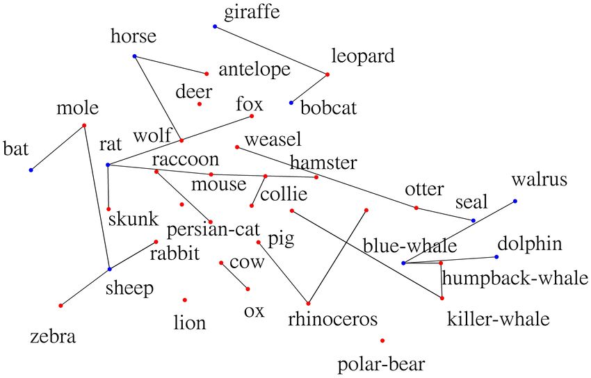
Published as a conference paper at ICLR 2021

(IPN)” to iteratively refine the prototypes by propagating them on a graph of classes so each
prototype is dynamically determined by the samples and attributes of its related classes.
In this section, we will first introduce the architecture of IPN. An illustration of IPN is given in
Figure 2. Then, we will elaborate the episodic training strategy, in which a consistency loss is
minimized for isometric alignment between the two spaces.

4.1    P ROTOTYPE I NITIALIZATION

Given a task T defined on a subset of classes Y T with training data DT , IPN first initializes the
semantic and visual prototype for each class y ∈ Y T . The semantic prototype of class y is trans-
formed from its attributes sy . Specifically, we have drawn on the expert modules from (Zhang &
Shi, 2019) to initialize the semantic prototypes Pys [0]. In previous works (Snell et al., 2017; Santoro
et al., 2016), the visual prototype of a class is usually computed by averaging the features of images
from the class. In IPN, for each seen class y ∈ Y T ∩ Y seen , we initialize its visual prototype Pyv [0]
by
                           W       X
                Pyv [0] = T                 fcnn (xi ), DyT , {(xi , yi ) ∈ DT : yi = y},            (1)
                          |Dy |           T
                                 (xi ,yi )∈Dy

where fcnn (·) is a backbone convolutional neural nets (CNN) extracting features from raw images,
and W is a linear transformation aiming to change the dimension of the visual prototype to be
the same as semantic prototypes. We argue that W is necessary because (1) the visual feature
produced by the CNN is usually in high dimension, and reducing its dimension can save significant
computations during propagation; (2) keeping the dimensions of the visual and semantic prototypes
the same can avoid the dominance of either of them in the model.
During test, we initialize the visual prototype of each unseen class y ∈ Y T ∩Y unseen as the weighted
sum of its K-nearest classes from Y seen in the semantic space1 , i.e.,
                                              X
                               Pyv [0] = W ·       as (Pys [0], Pzs [0]) · Pzv ,                   (2)
                                                z∈Ny

where W is the same transformation from Eq. (1), and Ny is the set of the top-K (K is a hyper-
parameter) seen classes2 with the largest similarities cs (Pys [0], Pzs [0]) to class y in semantic space.

4.2    C ATEGORY G RAPH G ENERATION

Although the propagation needs to be conducted on a category graph, IPN does not rely on any given
graph structure as many previous works (Kampffmeyer et al., 2019; Wang et al., 2018) so it has less
limitations when applied to more general scenarios. In IPN, we inference the category graph of Y T
by applying thresholding to the attention scores between the initialized prototypes. In the visual
space, the set of edges is defined by
                         E T,v = (y, z) : y, z ∈ Y T , cv (Pyv [0], Pzv [0]) ≥  ,

                                                                                                (3)
where  is the threshold. Thereby, the category graph is generated as G T,v = (Y T , E T,v ). Similarly,
in the semantic space, we generate another graph G T,s = (Y T , E T,s ).

4.3    I SOMETRIC P ROPAGATION

Given the initialized prototypes and generated category graphs in the two spaces, we apply the
following prototype propagation in each space for τ steps in order to refine the prototype of each
class. In the visual space, each propagation step updates
                                           X
                          Pyv [t + 1] =            av (Pyv [t], Pzv [t]) · Pzv [t],            (4)
                                           z:(y,z)∈E T ,v

   1
     This only happens in the test since we do not use any information of unseen classes during training.
   2
     Here the notation Ny needs a little overloading since it denotes the set of neighbor classes of y elsewhere
in the paper.

                                                            4
Published as a conference paper at ICLR 2021
In the semantic space, we apply similar propagation steps over classes on graph G T,s by using the
attention module associated with as (·, ·). Intuitively, the attention module computes the similarity
between the two prototypes. In the visual space, given the prototypes Pyv and Pzv for class y and z,
the attention module first computes the following cosine similarity:
hhv (Pyv ), hv (Pzv )i
cv (Pyv , Pzv ) = , (5)
khv (Pyv )k2 · khv (Pzv )k2
where hv (·) is a learnable transformation and k · k2 represents the `2 norm. For a class y on a
category graph, we can use the attention module to aggregate messages from its neighbor classes
Ny . In this case, we need to further normalize the similarities of y to each z ∈ Ny as follows.
exp[γcv (Pyv , Pzv )]
av (Pyv , Pzv ) = P v v v
, (6)
z∈Ny exp[γc (Py , Pz )]
where γ is a temperature parameter controlling the smoothness of the normalization. In the semantic
space, we have similar definitions of hs (·), cs (·, ·) and as (·, ·). In the following, we will use Pyv [t]
and Pys [t] to represent the visual and semantic prototype of class y at the tth step of propagation.
We will use | · | to represent the size of a set and ReLU(·) , max{·, 0}.
After τ steps of propagation, we concatenate the prototypes achieved in the two spaces for each
class to form the final prototypes:
Py = [Pyv [τ ], Pys [τ ]], ∀ y ∈ Y T . (7)
The formulation of as (·, ·) and cs (·, ·) follows the same way as av (·, ·) and cv (·, ·). To be simple,
we don’t rewrite the formulations here.
4.4 C LASSIFIER GENERATED FROM P ROTOTYPES
Given the final prototypes and a query/test image x, we apply a fully-connected layer to predict the
similarity between x and each class’s prototype. For each class y ∈ Y T , it computes
f (x, Py ) = w ReLU(W (1) x + W (2) Py + b(1) ) + b, (8)
Intuitively, the above classifier can be interpreted as a distance classifier with distance metric
f (·, ·). When applied to a query image x, the predicted class is the most probable class, i.e.,
ŷ = arg maxy∈Y T Pr(y|x; P ), where Pr denotes the probability.
4.5 T RAINING S TRATEGIES
Episodic training on subgraphs. In each episode, we sample a subset of training classes Y T ⊆
Y seen , and then build a training (or support) set Dtrain
T T
and a validation (or query) set Dvalid from
T
the training samples of Y . They are two disjoint sets of samples from the same subset of train-
T
ing classes. We only use Dtrain to generate the prototypes P by the aforementioned procedures,
T
and then apply backpropagation to minimize the loss of Dvalid . This equals to an empirical risk
minimization, i.e.,
X X
min − log Pr(y|x; P ), (9)
Y T ∼Y seen (x,y)∼Dvalid
T
This follows the same idea of meta-learning Ravi & Larochelle (2016): it aims to minimize the
validation loss instead of the training loss and thus can further improve generalization and restrain
overfitting. Moreover, since we train the IPN model on multiple random tasks T and optimize the
propagation scheme over different subgraphs (each generated for a random subset of classes), the
generalization capability of IPN to unseen classes and new tasks can be substantially enhanced by
this meta-training strategy. Moreover, it effectively reduces the propagation costs since computing
the attention needs O(|Y T |2 ) operations. In addition, as shown in the experiments, episodic train-
ing is effective in mitigating the problem of data imbalance and overfitting to seen classes, which
harasses many ZSL methods.
5Published as a conference paper at ICLR 2021
Consistency loss for alignment of visual and semantic space. In ZSL, the interaction and align-
ment between different spaces can provide substantial information about class dependency and is
critical to the generation of accurate class prototypes. In IPN, we apply prototype propagation in
two separate spaces on their own category graphs by using two untied attention modules. In order to
keep the propagation in the two spaces consistent, we add an extra consistency loss to the training
objective in Eq. (9). It computes the KL-divergence between two distributions defined in the two
spaces for each class y ∈ Y T at every propagation step t:
X psy [t]z
DKL (pvy [t]||psy [t]) = − pvy [t]z · log v , (10)
T
py [t]z
z∈Y
where
exp[cv (Pyv [t], Pzv [t])]
pvy [t]z , P v v v
, (11)
z∈Y T exp[c (Py [t], Pz [t])]
exp[cs (Pys [t], Pzs [t])]
psy [t]z , P s s s
. (12)
z∈Y T exp[c (Py [t], Pz [t])]
The consistency loss enforces the two attention modules in the two spaces to generate the same at-
tention scores over classes, even when the prototypes and attention module’s parameter are different
in the two spaces. In this way, they share similar class dependency over the propagation steps. So
the generated dual prototypes are well aligned and can provide complementary information when
generating the classifier. The final optimization we used to train IPN becomes:
X X X τ X
min − log Pr(y|x; P ) + λ DKL (pvy [t]||psy [t]) , (13)
Y T ∼Y seen T
(x,y)∼Dvalid t=1 y∈Y T
where λ is weight for the consistency loss, and P , pvy [t], and psy [t] are computed only based on
T
Dtrain , the training (or support) set of task-T for classes in Y T .
5 E XPERIMENTS
We evaluate IPN and compare it with several state-of-the-art ZSL models in both ZSL setting
(where the test set is only composed of unseen classes) and generalized ZSL setting (where the
test set is composed of both seen and unseen classes). We report three standard ZSL evaluation
metrics, and provide ablation study of several variants of IPN in the generalized ZSL setting. The
visualization of the learned class representation is shown in Figure 1.
5.1 DATASETS AND E VALUATION CRITERIA
Small and Medium benchmarks. Our evaluation includes experiments on three standard bench-
mark datasets widely used in previous works, i.e., AWA2 (Xian et al., 2019a), CUB (Welinder et al.,
2010) and aPY (Farhadi et al., 2009). The former two are extracted from ImageNet-1K, where
AWA2 contains 50 animals classes and CUB contains 200 bird species. aPY includes 32 classes.
Detailed statistics of them can be found in Table 1.
Two new large-scale benchmarks. The three benchmark datasets above might be too small for
modern DNN models since the training may suffers from large variance and end-to-end training
usually fails. Previous ZSL methods therefore fine-tune a pre-trained CNN to achieve satisfactory
performance on these datasets, which is costly and less practical. Given these issues, we proposed
two new large-scale datasets extracted from tieredImageNet (Ren et al., 2018), i.e., tieredImageNet-
Segregated and tieredImageNet-Mixed, whose statistics are given in Table 1. Comparing to the
three benchmarks, they are over 10× larger, and training a ResNet101 (He et al., 2016) from scratch
on their training sets can achieve a validation accuracy of 65%, indicating that end-to-end training
without fine-tuning is possible. These two benchmarks differ in that the “Mixed” version allows
a seen class and an unseen class to belong to the same super category, while the “Segregated”
version does not. The class attributes are the word embeddings of the class names provided by
GloVe (Pennington et al., 2014). We removed the classes that do not have embeddings in GloVe.
Following the most popular setting of ZSL (Xian et al., 2019a), we report the per-class accuracy and
harmonic mean of the accuracy on seen and unseen classes.
6Published as a conference paper at ICLR 2021
Dataset #Attributes #Seen #Unseen #Imgs(Tr-S) #Imgs(Te-S) #Imgs(Te-U)
CUB (Welinder et al., 2010) 312 150 50 7,057 1,764 2,967
AWA2 (Xian et al., 2019a) 85 40 10 23,527 5,882 7,913
aPY (Farhadi et al., 2009) 64 20 12 5,932 1,483 7,924
tieredImageNet-Segregated 300 422 182 378,884 162,952 232,129
tieredImageNet-Mixed 300 447 157 399,741 171,915 202,309
Table 1: Datasets Statistics. CUB, AWA2 and aPY are three standard ZSL benchmarks, while
tieredImageNet-Segregated/Mixed are two new large-scale ones proposed by us with different dis-
crepancy between seen and unseen classes. “Tr-S”, “Te-S” and “Te-U” denote seen classes in train-
ing, seen classes in test and unseen classes in test.
CUB AWA2 aPY tiered-M tiered-S
Methods
S U H S U H S U H S U H S U H
GDAN 66.7 39.3 49.5 67.5 32.1 43.5 75.0 30.4 43.4 50.5 2.1 4.0 3.9 1.2 1.8
LisGAN 57.9 46.5 51.6 76.3 52.6 62.3 68.2 34.3 45.7 1.6 0.1 0.2 0.2 0.1 0.1
Generative
CADA-VAE 53.5 51.6 52.4 75.0 55.8 63.9 - - - 60.1 3.5 6.5 0.8 0.1 0.2
Models
f-VAEGAN-D2 60.1 48.4 53.6 70.6 57.6 63.5 - - - - - - - - -
FtFT 54.8 47.0 50.6 72.6 55.3 62.6 - - - - - - - - -
Relation Net 61.1 38.1 47.0 93.4 30.0 45.3 - - - 31.4 3.4 6.1 45.8 1.2 2.3
GAFE 52.1 22.5 31.4 78.3 26.8 40.0 68.1 15.8 25.7 - - - - - -
PQZSL 51.4 43.2 46.9 - - - 64.1 27.9 38.8 - - - - - -
Discriminative MLSE 71.6 22.3 34.0 83.2 23.8 37.0 74.3 12.7 21.7 - - - - - -
Models CRNet 56.8 45.5 50.5 78.8 52.6 63.1 68.4 32.4 44.0 58.0 2.5 4.9 57.6 1.0 2.0
TCN 52.0 52.6 52.3 65.8 61.2 63.4 64.0 24.1 35.1 - - - - - -
RGEN 73.5 60.0 66.1 76.5 67.1 71.5 48.1 30.4 37.2 - - - - - -
APN 55.9 48.1 51.7 83.9 54.8 66.4 74.7 32.7 45.5 - - - - - -
IPN (ours) 73.8 60.2 66.3 79.2 67.5 72.9 66.0 37.2 47.6 50.1 6.1 11.0 54.4 2.5 4.7
Table 2: Performance of existing ZSL models and IPN on five datasets (generalized ZSL setting),
where “S” denotes the per-class accuracy (%) on seen classes, “U” denotes the per-class accuracy
(%) on unseen classes and “H” denotes their harmonic mean.
5.2 I MPLEMENTATION AND H YPERPARAMETER D ETAILS
For a fair comparison, we follow the setting in (Xian et al., 2019a) and use a pre-trained ResNet-
101 (He et al., 2016) to extract 2048-dimensional image features without fine-tuning. For the three
standard benchmarks, the model is pre-trained on ImageNet-1K. For the two new datasets, it is
pre-trained on the training set used to train ZSL models.
All hyperparameters were chosen on the validation sets provided by Xian et al. (2019a). We use the
same hyperparameters tuned on AWA2 for other datasets since they are of similar data type, except
for aPY on which we choose learning rate 1.0 × 10⁻³ and weight decay 5.0 × 10⁻⁴ . For the rest of
the datasets, we train IPN by Adam (Kingma & Ba, 2015) for 360 epochs with a weight decay factor
1.0 × 10⁻⁴ . The learning rate starts from 2.0 × 10⁻⁵ and decays by a multiplicative factor 0.1 every
240 epochs. In each epoch, we update IPN on multiple N -way-K-shot tasks (N -classes with K
samples per class), each corresponding to an episode mentioned in Section 4.5. In our experiments,
the number of episodes in each epoch is n/N K , where n is the total size of the training set, N = 30
and K = 1 (a small K can mitigate the imbalance between seen and unseen classes); hv and hs are
linear transformations; we set temperature γ = 10, threshold = cos 40o for the cosine similarities
between class prototypes, and weight for consistency loss λ = 1. We use propagation steps τ = 2.
5.3 M AIN R ESULTS
The results are reported in Table 2. Although most previous works (Xian et al., 2019b;a; Sariyildiz
& Cinbis, 2019) show that the more complicated generative models usually outperforms the discrim-
inative ones. Our experiments imply that IPN, as a simple discriminative model, can significantly
outperform the generative models requiring much more training efforts. Most baselines achieve a
7Published as a conference paper at ICLR 2021
high ACCseen but much lower ACCunseen since they suffer from and more sensitive to the imbal-
ance between seen and unseen classes. In contrast, IPN always achieves the highest H-metric among
all methods, indicating less overfitting to seen classes. This is due to the more accurate prototypes
achieved by iterative propagation in two interactive spaces across seen and unseen classes, and the
episodic training strategy, which effectively improves the generalization.
In scaling the experiments to the two large datasets, discriminative models perform better than gen-
erative models, which are easily prone to overfitting or divergence. Moreover, during the test stage,
generative models require to synthesize data for unseen classes, which may lead to expensive compu-
tations when applied to tasks with many classes. In contrast, IPN scales well to these large datasets,
outperforming state-of-the-art baselines by a large margin. The performance of most models on
tieredImageNet-Segregated is generally worse than tieredImageNet-Mixed because that the unseen
classes in the former do not share the same ancestor classes with the seen classes, while in the latter
such sharing is allowed.
5.4 A BLATION S TUDY
Are two prototypes necessary? We compare IPN with its two variants, each using only one out of
the two types of prototypes from the two spaces when generating the classifier. The results are shown
in Figure 3. It shows that semantic prototype (only) performs much better than visual prototype
(only), especially on the unseen classes. This is because that the unseen classes’ semantic embedding
is given while its visual information is missing (zero images) during the test stage. Although IPN is
capable of generating a visual prototype based on other classes’ images and class dependency, it is
much less accurate than the semantic prototype. However, it also shows that the visual prototypes
(even the ones of unseen classes) can provide extra information and further improve the performance
of the semantic prototype, e.g., they improve the unseen classes’ accuracy from 61.1% to 67.5%.
One possible reason is that the visual prototype bridges the query image’s visual feature with the
semantic features of classes, and thus provides an extra “visual context” for the localization of the
correct class. In addition, we observe that IPN with only the visual prototype converges faster than
IPN with only a semantic prototype (30 epochs vs. 200 epochs). This might be an artifact caused
by the pre-trained CNN, which already produces stable visual prototypes since the early stages.
However, it raises a caveat that heavily relying on a pre-trained model might discourage the learning
and results in a bad local optimum.
S U H S U H S U H
90 100 90
75
60 60
50
30 30
25
0 0 0
Semantic Visual Visual + Semantic Semantic Visual Visual + Semantic Semantic Visual w/o Consistency
Effect of Prototypes Effect of Propagation Effect of Isometric Alignment
Figure 3: Ablation study of IPN on AWA2 (generalized ZSL setting). “S”, “U” and “H” are the
same notations used in Table 2. (a) Only one of the dual prototypes are used to generate classifiers.
(b) Only one or none of the propagation in the two spaces are applied in IPN. (c) Different types of
interaction between spaces. “visual/semantic attention only” means we use visual/semantic attention
in both spaces, “two separate attentions” refers to IPN trained without consistency loss.
How’s the benefit of propagation? We then evaluate the effects of the propagation scheme in the
two spaces. In particular, we compare IPN with its variants that apply the propagation steps in only
one of the two spaces, and the variant that does not apply any propagation after initialization. Their
performance is reported in Figure 3. Without any propagation, the classification performance heav-
ily relies on pre-trained CNN. Hence, the accuracy of seen classes can be much higher than that
of the unseen classes. Compared to IPN without any propagation, applying propagation in either
the visual space or the semantic space can improve the accuracy of unseen classes by 2∼3%, while
the accuracy on the seen classes stays almost the same. When equipped with dual propagation, we
8Published as a conference paper at ICLR 2021
observe a significant improvement of the accuracy of the unseen classes but a degradation on the
seen classes. However, they lead to the highest H-metric, which indicates that the dual propaga-
tion achieves a desirable trade-off between overfitting on seen classes and generalization to unseen
classes.
Effect of Isometric Alignment In IPN, we minimize a consistency loss during training for align-
ment of the visual and semantic space. Here, we consider two other options for alignment that
exchange the attention modules used in the two spaces, i.e., using the visual attention module in
the semantic space, or using the semantic attention module in the visual space. We also include the
IPN trained without consistency loss or any alignment as a baseline. Their results are reported in
Figure 3. Compared to IPN with/without consistency loss, sharing a single attention module be-
tween the two spaces suffers from the overfitting problem on the seen classes. This is because that
the visual features and semantic embeddings are two different types of features so they should not
share the same similarity metric. In contrast, the consistency loss only enforces the output similarity
scores of the two attention modules to be close, while the models/functions computing the similarity
can be different. Therefore, to produce the same similarity scores, it does not require each class
having the same features in the two spaces. Hence, it leads to a much softer regularization.
6 S ENSITIVITY OF HYPERPARAMETERS
73.0
70 72
the harmonic mean
60 72.5
70
50 72.0 non-episodic
40 68
71.5
30 66
71.0
20
64
20 30 40 50 60 70 80 90 0 5 10 15 20 25 30 0 1 2 3 4 5
the threshold ( ) the temperature ( ) The value of K (30-way-K-shot)
73.0 72.5 73
72.5 70.0 72
the harmonic mean
72.0 67.5 71
71.5 65.0 70
71.0 62.5 69
70.5 60.0 68
67
70.0 non-episodic 57.5
66
0 5 10 15 20 25 30 35 40 0 1 2 3 4 5 2.0e4 4.0e4 6.0e4 8.0e4 10.0e4
The value of N (N-way-1-shot) The propagation steps ( ) The weight decay
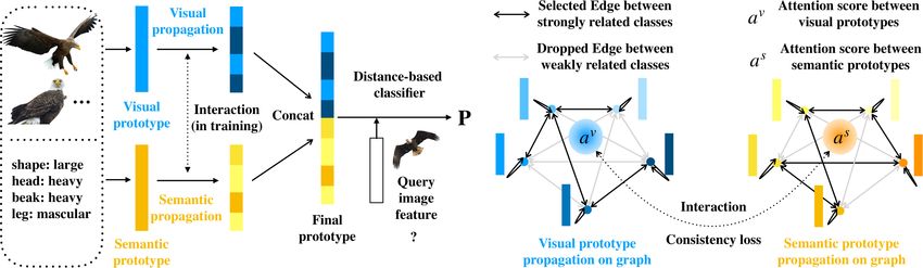
Figure 4: Performance analysis when using different values of hyperparameters on AWA2.
The proposed IPN has some hyperparameters as mentioned in Section 5.2. To analyze the sensi-
tivity of those hyperparameters, such as threshold, temperature, N and K for N-way-K-shot task,
propagation steps, etc. We try different values and show the performance on the AWA2 dataset in
Figure 4. The temperature γ is not sensitive for the accuracy. The threshold needs to be bigger than
cosine(30o ) to give IPN some space for the filtering. The propagation steps τ is best at 2. Weight
decay is a sensitive hyperparameter and this is also found in previous ZSL literature (Zhang & Shi,
2019; Liu et al., 2019d).
7 C ONCLUSIONS
In this work, we propose an Isometric Propagation Network, which learns to relate classes within
each space and across two spaces. IPN achieves state-of-the-art performance and we show the
importance of each component and visualize the interpretable relationship of the learned class rep-
resentations. In future works, we will study other possibilities to initialize the visual prototypes of
unseen classes in IPN.
9Published as a conference paper at ICLR 2021
R EFERENCES
Zeynep Akata, Florent Perronnin, Zaid Harchaoui, and Cordelia Schmid. Label-embedding for
image classification. TPAMI, 2015a. doi: 10.1109/TPAMI.2015.2487986.
Zeynep Akata, Scott Reed, Daniel Walter, Honglak Lee, and Bernt Schiele. Evaluation of output
embeddings for fine-grained image classification. In CVPR, 2015b.
Yannick Le Cacheux, Herve Le Borgne, and Michel Crucianu. Modeling inter and intra-class rela-
tions in the triplet loss for zero-shot learning. In ICCV, 2019.
Soravit Changpinyo, Wei-Lun Chao, Boqing Gong, and Fei Sha. Synthesized classifiers for zero-
shot learning. In CVPR, 2016.
Soravit Changpinyo, Wei-Lun Chao, and Fei Sha. Predicting visual exemplars of unseen classes for
zero-shot learning. In ICCV, 2017.
Haoang Chi, Feng Liu, Wenjing Yang, Long Lan, Tongliang Liu, Gang Niu, and Bo Han. Meta
discovery: Learning to discover novel classes given very limited data, 2021.
Kaize Ding, Jianling Wang, Jundong Li, Kai Shu, Chenghao Liu, and Huan Liu. Graph proto-
typical networks for few-shot learning on attributed networks. In Proceedings of the 29th ACM
International Conference on Information & Knowledge Management, 2020.
Kaize Ding, Qinghai Zhou, Hanghang Tong, and huan Liu. Few-shot network anomaly detection
via cross-network meta-learning. In Proceedings of The Web Conference 2021, 2021.
Xuanyi Dong and Yi Yang. Searching for a robust neural architecture in four gpu hours. In CVPR,
2019.
Xuanyi Dong, Lu Liu, Katarzyna Musial, and Bogdan Gabrys. NATS-Bench: Benchmarking nas
algorithms for architecture topology and size. TPAMI, 2021. doi: 10.1109/TPAMI.2021.3054824.
Hehe Fan, Ping Liu, Mingliang Xu, and Yi Yang. Unsupervised visual representation learning
via dual-level progressive similar instance selection. TCYB, 2021. doi: 10.1109/TCYB.2021.
3054978.
Ali Farhadi, Ian Endres, Derek Hoiem, and David Forsyth. Describing objects by their attributes. In
CVPR, 2009.
Chelsea Finn, Pieter Abbeel, and Sergey Levine. Model-agnostic meta-learning for fast adaptation
of deep networks. In ICML, 2017.
Andrea Frome, Greg S Corrado, Jon Shlens, Samy Bengio, Jeff Dean, Tomas Mikolov, et al. Devise:
A deep visual-semantic embedding model. In NeurIPS, 2013.
Ian Goodfellow, Jean Pouget-Abadie, Mehdi Mirza, Bing Xu, David Warde-Farley, Sherjil Ozair,
Aaron Courville, and Yoshua Bengio. Generative adversarial nets. In NeurIPS, 2014.
Kaiming He, Xiangyu Zhang, Shaoqing Ren, and Jian Sun. Deep residual learning for image recog-
nition. In CVPR, 2016.
He Huang, Changhu Wang, Philip S Yu, and Chang-Dong Wang. Generative dual adversarial net-
work for generalized zero-shot learning. In CVPR, 2019.
Huajie Jiang, Ruiping Wang, Shiguang Shan, and Xilin Chen. Learning class prototypes via structure
alignment for zero-shot recognition. In ECCV, 2018.
Michael Kampffmeyer, Yinbo Chen, Xiaodan Liang, Hao Wang, Yujia Zhang, and Eric P Xing.
Rethinking knowledge graph propagation for zero-shot learning. In CVPR, 2019.
Diederik P Kingma and Jimmy Ba. Adam: A method for stochastic optimization. In ICLR, 2015.
Elyor Kodirov, Tao Xiang, and Shaogang Gong. Semantic autoencoder for zero-shot learning. In
CVPR, 2017.
10Published as a conference paper at ICLR 2021
Christoph H Lampert, Hannes Nickisch, and Stefan Harmeling. Attribute-based classification for
zero-shot visual object categorization. TPAMI, 2014. doi: 10.1109/TPAMI.2013.140.
Hugo Larochelle, Dumitru Erhan, and Yoshua Bengio. Zero-data learning of new tasks. In IJCAI,
2008.
Jingjing Li, Mengmeng Jin, Ke Lu, Zhengming Ding, Lei Zhu, and Zi Huang. Leveraging the
invariant side of generative zero-shot learning. In CVPR, 2019a.
Kai Li, Martin Renqiang Min, and Yun Fu. Rethinking zero-shot learning: A conditional visual
classification perspective. In CVPR, 2019b.
Yanan Li, Donghui Wang, Huanhang Hu, Yuetan Lin, and Yueting Zhuang. Zero-shot recognition
using dual visual-semantic mapping paths. In CVPR, 2017.
Feng Liu, Wenkai Xu, Jie Lu, Guangquan Zhang, Arthur Gretton, and Danica J. Sutherland. Learn-
ing deep kernels for non-parametric two-sample tests. In ICML, volume 119, pp. 6316–6326,
2020.
Lu Liu, Tianyi Zhou, Guodong Long, Jing Jiang, Lina Yao, and Chengqi Zhang. Prototype prop-
agation networks (PPN) for weakly-supervised few-shot learning on category graph. In IJCAI,
2019a.
Lu Liu, Tianyi Zhou, Guodong Long, Jing Jiang, and Chengqi Zhang. Learning to propagate for
graph meta-learning. In NeurIPS, 2019b.
Shichen Liu, Mingsheng Long, Jianmin Wang, and Michael I Jordan. Generalized zero-shot learning
with deep calibration network. In NeurIPS, 2018.
Yang Liu, Jishun Guo, Deng Cai, and Xiaofei He. Attribute attention for semantic disambiguation
in zero-shot learning. In ICCV, 2019c.
Yang Liu, Deyan Xie, Quanxue Gao, Jungong Han, Shujian Wang, and Xinbo Gao. Graph and
autoencoder based feature extraction for zero-shot learning. In IJCAI, 2019d.
Yixin Liu, Shirui Pan, Ming Jin, Chuan Zhou, Feng Xia, and Philip S. Yu. Graph self-supervised
learning: A survey, 2021.
Laurens van der Maaten and Geoffrey Hinton. Visualizing data using t-SNE. JMLR, 2008.
Mohammad Norouzi, Tomas Mikolov, Samy Bengio, Yoram Singer, Jonathon Shlens, Andrea
Frome, Greg S Corrado, and Jeffrey Dean. Zero-shot learning by convex combination of semantic
embeddings. In NeurIPS, 2013.
Jeffrey Pennington, Richard Socher, and Christopher Manning. Glove: Global vectors for word
representation. In EMNLP, 2014.
Sachin Ravi and Hugo Larochelle. Optimization as a model for few-shot learning. In ICLR, 2016.
Mengye Ren, Eleni Triantafillou, Sachin Ravi, Jake Snell, Kevin Swersky, Joshua B Tenenbaum,
Hugo Larochelle, and Richard S Zemel. Meta-learning for semi-supervised few-shot classifica-
tion. In ICLR, 2018.
Bernardino Romera-Paredes and Philip Torr. An embarrassingly simple approach to zero-shot learn-
ing. In ICML, 2015.
Adam Santoro, Sergey Bartunov, Matthew Botvinick, Daan Wierstra, and Timothy Lillicrap. Meta-
learning with memory-augmented neural networks. In ICML, 2016.
Mert Bulent Sariyildiz and Ramazan Gokberk Cinbis. Gradient matching generative networks for
zero-shot learning. In CVPR, 2019.
Jake Snell, Kevin Swersky, and Richard Zemel. Prototypical networks for few-shot learning. In
NeurIPS, 2017.
11Published as a conference paper at ICLR 2021
Richard Socher, Milind Ganjoo, Christopher D Manning, and Andrew Ng. Zero-shot learning
through cross-modal transfer. In NeurIPS, 2013.
Robyn Speer, Joshua Chin, and Catherine Havasi. Conceptnet 5.5: An open multilingual graph of
general knowledge. arXiv preprint arXiv:1612.03975, 2016.
Flood Sung, Yongxin Yang, Li Zhang, Tao Xiang, Philip HS Torr, and Timothy M Hospedales.
Learning to compare: Relation network for few-shot learning. In CVPR, 2018.
Bin Tong, Chao Wang, Martin Klinkigt, Yoshiyuki Kobayashi, and Yuuichi Nonaka. Hierarchical
disentanglement of discriminative latent features for zero-shot learning. In CVPR, 2019.
Xiaolong Wang, Yufei Ye, and Abhinav Gupta. Zero-shot recognition via semantic embeddings and
knowledge graphs. In CVPR, 2018.
Peter Welinder, Steve Branson, Takeshi Mita, Catherine Wah, Florian Schroff, Serge Belongie, and
Pietro Perona. Caltech-ucsd birds 200. Technical report, California Institute of Technology, 2010.
Yongqin Xian, Christoph H Lampert, Bernt Schiele, and Zeynep Akata. Zero-shot learning-a com-
prehensive evaluation of the good, the bad and the ugly. TPAMI, 2019a. doi: 10.1109/TPAMI.
2018.2857768.
Yongqin Xian, Saurabh Sharma, Bernt Schiele, and Zeynep Akata. f-vaegan-d2: A feature generat-
ing framework for any-shot learning. In CVPR, 2019b.
Guo-Sen Xie, Li Liu, Xiaobo Jin, Fan Zhu, Zheng Zhang, Jie Qin, Yazhou Yao, and Ling Shao.
Attentive region embedding network for zero-shot learning. In CVPR, 2019.
Guo-Sen Xie, Li Liu, Fan Zhu, Fang Zhao, Zheng Zhang, Yazhou Yao, Jie Qin, and Ling Shao.
Region graph embedding network for zero-shot learning. In CVPR, 2020.
Fei Zhang and Guangming Shi. Co-representation network for generalized zero-shot learning. In
ICML, 2019.
Li Zhang, Tao Xiang, and Shaogang Gong. Learning a deep embedding model for zero-shot learning.
In CVPR, 2017.
Pengkai Zhu, Hanxiao Wang, and Venkatesh Saligrama. Generalized zero-shot recognition based
on visually semantic embedding. In CVPR, 2019a.
Yizhe Zhu, Jianwen Xie, Zhiqiang Tang, Xi Peng, and Ahmed Elgammal. Semantic-guided multi-
attention localization for zero-shot learning. In NeurIPS, 2019b.
A E VALUATION C RITERIA
Considering the imbalance between test classes, by following the most recent works (Xian et al.,
2019a), given a test set D, we evaluate ZSL methods’ performance based on the per-class accuracy
averaged over a targeted set of classes Y, i.e.,
1 X 1
1[by = y],
X
ACCY = (14)
|Y| |Dy |
y∈Y (x,y)∈Dy
Dy , {(xi , yi ) ∈ D : yi = y}.
Following Xian et al. (2019a), we report ACCY when Y = Yseen and Y = Yunseen , and the
harmonic mean of them, i.e.,
2 · ACCYseen · ACCYunseen
H= . (15)
ACCYseen + ACCYunseen
12Published as a conference paper at ICLR 2021
Methods CUB AWA2 aPY tiered-M tiered-S
Generative LisGAN (Li et al., 2019a) 58.8 70.6 43.1 1.6 0.1
Models f-VAEGAN-D2 (Xian et al., 2019b) 61.0 71.1 - - -
SAE (Kodirov et al., 2017) 33.3 54.1 8.3 - -
DEM (Zhang et al., 2017) 51.7 67.1 35.0 - -
Discriminative RN (Sung et al., 2018) 55.6 64.2 30.1 6.1 2.5
Models GAFE (Liu et al., 2019d) 52.6 67.4 44.3 - -
IPN (ours) 59.6 74.4 42.3 14.0 5.0
Table 3: Per-class accuracy (%) on unseen classes achieved by existing ZSL models and IPN on five
datasets (the ZSL setting).
B E XPERIMENTS ON Z ERO - SHOT L EARNING SETTING
The comparison between IPN to other baselines on the setting of Zero-shot Learning is shown in
Table 3. On CUB, AWA2, aPU, tiered-M, and tiered-S, our IPN outperforms other algorithms by a
large margin.
C M ORE E XPERIMENTS ON L ARGE - SCALE DATASETS
In our work, we follow the train/test split suggested by Frome et al. (2013), who proposed to use the
21K ImageNet dataset for zero-shot evaluation. Here, 2-hops and 3-hops represent that the evalua-
tion is over the classes which are 2/3 hops away from ImageNet-1k. Different from experiments on
AWA2, we use N =20 and K=5 for the full ImageNet. Besides, since the edges between each class
are provided on the full ImageNet, we directly use them instead of calculating by Eq. (3).
Hit@k (%) [2-hops] Hit@k (%) [3-hops]
Methods
1 5 10 20 1 5 10 20
ConSE (Norouzi et al., 2013) 8.3 21.8 30.9 41.7 2.6 7.3 11.1 16.4
SYNC (Changpinyo et al., 2016) 10.5 28.6 40.1 52.0 2.9 9.2 14.2 20.9
EXEM (Changpinyo et al., 2017) 12.5 32.3 43.7 55.2 3.6 10.7 16.1 23.1
GCNZ (Wang et al., 2018) 19.8 53.2 65.4 74.6 4.1 14.2 20.2 27.7
DGP (Kampffmeyer et al., 2019) 26.6 60.3 72.3 81.3 6.3 19.3 27.7 37.7
IPN (ours) 27.1 61.1 73.8 82.9 6.8 20.1 28.9 39.6
Table 4: Top-k accuracy for the different models on the ImageNet dataset. Accuracy when only
testing on unseen classes. Results are taken from (Kampffmeyer et al., 2019).
13You can also read