Laetitia Le Pourhiet - Tectonic modelling state of the art and future challenges an introduction to Analogue and numerical modelling of tectonic ...

Tectonic modelling state of the art and future challenges

an introduction to Analogue and numerical modelling of tectonic processes
 vEGU2021

 Laetitia Le Pourhiet

2

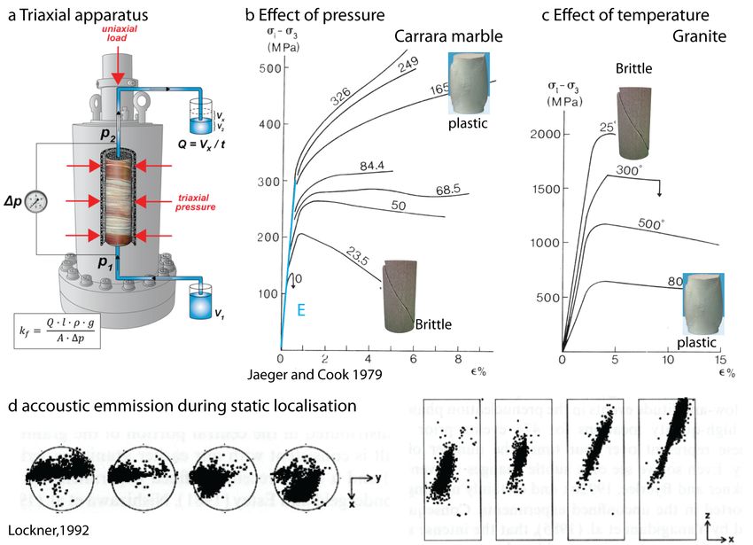
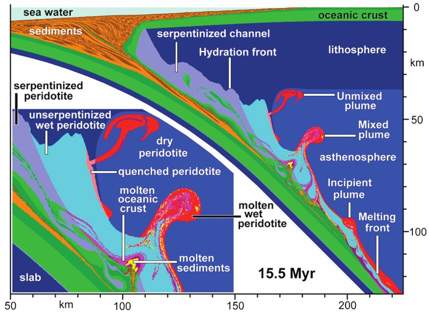
30 million particles of distinct density used to represent strength” of the upper layer (thickness, angl
 the two fluids. The thermal case was modelled using cohesion) relative to that of the lower laye
 160 × 160 × 320elements—a significantly higher res- systematic change in the characteristic sp
 At lithospheric scale industry codes do not work ! So many codes have
 olution needed to resolve the extremely fine thermal
 boundary layer which develops around the conduit; in
 shear bands (Montesi and Zuber, 2000; Hui
 2005).
 emerge in the community
 this example the transition to unstable behaviour has not The principal challenge in 3D is to achiev
 yet been reached. As the thermal diffusivity is reduced ful resolution, given the very large number
 further, the thermal boundary layer will become thin- mesh points, and the additional degree of fre
 ner still and a finer mesh resolution will be required to mesh point. Fig. 5 shows a comparison betw
 resolve its structure.10 However, we know from analysis of of the Earth and Planetary Interiors xxx (2011) xxx–xxx
 C. Thieulot / Physics

 the non-diffusing limit that no further(Thieulot, PEPI,of
 refinement 2011) the
20-120 Millions d’années

 velocity mesh is required to resolve the developing insta-
 bility. In order to determine
 (a) the point at which diffusion (b)
 is no longer able to suppress the growth of the instability
 in the conduit, we plan to refine only the mesh for the
 energy equation. (c) (d)

 6.2. Basin extension model

 The following models (e) are motivated by a prelimi- (f )
 nary study of the difference between 2D and 3D studies
 of basin-forming processes in extending lithosphere
 (Moresi et al., 2007). Two-dimensional models are well
 understood, and, with(g)sufficient resolution, can be reli- (h)
 ably reproduced using different numerical techniques
 (Buiter et al., 2006). Some uncertainty remains, however,
 in application of 2D models to both real geological set-
 tings and analogue laboratory
 (i) experiments designed to (j)
 illuminate the geology; the formation of truly 3D struc-
 (Moresi et al, PEPI, 2007)
 ture cannot be understood from
 Fig. 7. Numerical sandboxpurely
 experiments2D experiments.
 results at low resolution (left column) and high resolution (right column) after 2 cm of extension. (a and b) Materials
 Fig. 4.scale),
 The extension ofcomponent
 a viscoplastic layer overlying
 Fig. 4 shows 2 ×rate2(logarithmic
 × 1 box (96 × 96 × 48 elements)
 scale), (e and f) pressure, (g and h) effective viscosity (logarithmic (i and j) horizontal of the velocity field.

 strate for a range of values of the cohesion of the viscop
 large displacements extending in the x1advection
 direction
 of 1, in which a viscoplastic
 at a dimensionless velocity
 of the cloud points takes 0.034 s in the low resolution
 case and 0.4 slayer with a Mohr-Coulomb
 in the high-resolution one. In both cases, these oper-
 shear bands Thewhich
 setup,develop
 shown inhave
 Fig. 8,been
 where they meet the free surface and the edge of th
 highlighted
 consists by
 of three layer

 ations represent only a fraction of the solving time and of the total ! The top layer is the crust, consisting of wet quart
 failure model as described by (18) with η = 10, tan ϕ =
 non linear mechanical behaviour running time.
 FANTOM allows for the accurate tracking of the amount of
 memory that it allocates all through the run (outside of the solver).
 output movies thickfor reference.
 and is characterised by a visco-plastic r
 2800 kg m"3, cqt = 20 # 106 Pa, nqt = 4.0, Qqt = 223
 Aqt = 1.10 # 10"28 Pa"n s"1, Vqt = 0 m3 mol"1, / =

 short time steps and long term simulations In the low resolution case, it does not exceed 30 Mb, and in the
 high resolution case 520 Mb. Given the amount of memory avail-
 able on which the code is set to run (typically between 2 and
 !1 = 0.5, !2 = 1.5.
 ! The middle layer is the lithosphere and sublithosp
 composed of dry olivine. It is 85 km thick and it
 32 Gb on modern desktop computers), this allows to assess how also visco-plastic. q0 = 3300 kg m"3, col = 20 # 10

 strong coupling (mechanics, thermal, thermo-dynamics much memory is left available to the direct solver, whose memory
 needs are difficultly predictible.
 Qol = 540 # 103 J mol"1, Aol = 2.4168 # 10"15 Pa"n s
 10"6 m3 mol"1, / = 7!, /sw = 1!, !1 = 0.5, !2 = 1.5.

 erosion and sedimentation, deep fluid flow) In the low resolution case, the measured dip angles are about
 53 ± 2! on each side, while in the high resolution case the mea-
 ! The bottom layer is the mantle, characterised by
 cous rheology. q0 = 3300 kg m"3, l = 1021 Pa s.
 sured dip angles are 54 ± 1! on each side and are therefore steeper.

 3D In both cases, the measurements are within the values expected for
 pressure-dependent non-dilational Mohr–Coulomb shear zones
 (Kaus, 2010).
 The size of the numerical domain is Lx = 1200 km
 and the boundary conditions are as follows: the te
 set to T = 1330 !C at the base of the model and to 0
 Finally, an observation can be made about the density of the At startup, a constant geotherm T = 550 !C is place
 shear band network which grows with each increase in resolution: of the crust.
 sandbox experiments do not show such a high density network of (Gorczyk, et al, 2007; Gerya, 2011)
 The extensional velocity applied to the sides o
 shear band and this probably implies that the implemented plastic vext = 0.5 cm yr"1 and a re-entrant velocity field is a
 rheology is too simple and lacks constitutive parameters defining rest of the boundary so as to lead to a zero net-flux
 the band spacing (Chemenda, 2007). vertical sides of the box. A weak seed is placed in th

All these code share a lot of similarities

 determined from experimental data

 viscosity, density are the coefficients

 Z d
 X and thermodynamic
A(u, v) = 2⌘ Dij (u)Dij (v) dV, models
 ⌦ i,j=1
 Z Z
 F (v) = v · f dV + v · t̄ dS.
 ⌦ N

 Thermal coupling and non linear constitutives equations lead to
 viscosity variations of 6 to 8 orders of magnitude

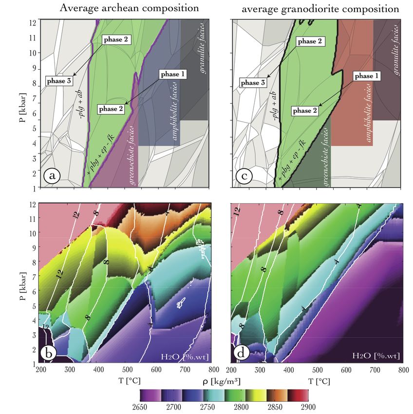
These models can then be coupled to
 fluid flow, and surface process models, earthquakes

 @
 2%wt H20
 4%wt H20

 0 Fluid fraction % 100

 Mezri et al. 2015 lithos Plunder et al . submitted

 Perron et al. 2021 BSGF
dal zilio et al. 2018 EPSL

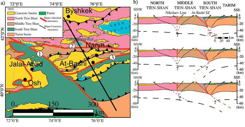
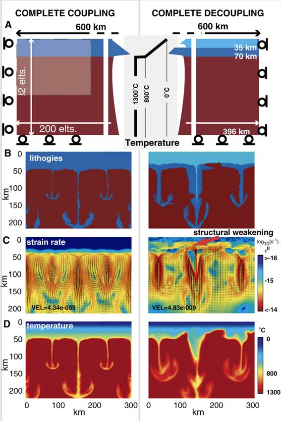
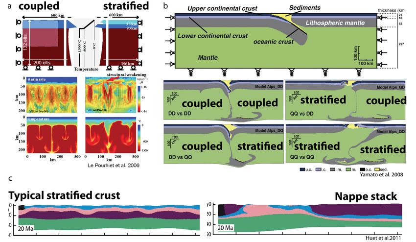
For a long time numerical simulations served to test the impact of the
 rheology of the crust on the rheology of the lithosphere mostly in 2D.

coupled stratified
 coupled stratified
 extension mode

 coupled stratified

 Narrow rift Wide rift
 S. DYKSTERHUIS et al 2007Geological Society of London

 collision mode
 Thèse P. Yamato

Le Pourhiet et al. EPSL, 2006

 Lithospheric stability
 Yamato et al. JGR, 2008

I consider those problems as solved
and we should not be solving them again and again

Yet emergence of 3D models might change a little bit these views

 coupled stratified
n mode

 Narrow Wide

 stratified Narrow rift coupe

 S. DYKSTERHUIS et al 2007Geological Society of London carte

 In 3D, continental break up
 coupled stratified propagation can be 10 times
 faster than stretching stratified Wide rift coupe

 Narrow rift can form in
 stratified lithosphere
 carte

 Le Pourhiet et al., Nature Geosciences, 2018

Now model can be used to test hypothesis
 how to draw a lithospheric scale cross section ?

 Several hypothesis concerning the Tien Shan belt at depth NNW NORTH TIEN-SHAN MIDDLE TIEN-SHAN SOUTH TIEN-SHAN TARIM SSE
 based on different possible inherited structures from the Nikolaev Line At-Bashi SZ
 4 4
 Paleozoic 0 0
 -8 -8
 -16 -16
 -24 -24
 -32 -32
 -40 -40
 -48 -48
 -56 -56
 (km) km (km)
 0 20 40

 NORTH TIEN-SHAN MIDDLE TIEN-SHAN SOUTH TIEN-SHAN
 Paleozoic cover Paleozoic cover High pressure micaschists
 Ordovician plutons + basement Basement Accretionary wedge
 TARIM
 Paleozoic cover Cenozoic cover Lower crust
 Basement Permian granites

 And Finally build a lithospheric cross-section constrained
 by mechanical models

Modellin permits to test the different hypothesis on the Kyrgyz Naryn At Bashi Aksai Tarim
 structure of the crust 30 Ma ago N range Basin range Basin S
 a
 -20
 a) Run 1 Free Surface Sediments - 5 Km (Quartz)
 0.25 mm/yr 40 Km
 120 Km

 Upper crust - 20 Km (Quartz) -40
 300 Km

 0.25 mm/yr

 Lower crust - 20 Km (Diorite)
 1300 °C
 75 elts

 -60
 Nikolaev Line 15 Km (Quartz)
 At-Bashi Suture zone - 30 Km
 800 Km 50 100 150 200 250 300 350 km

 0.25 mm/yr
 200 elts (Schist)
 Mantle (dry olivine)
 To compare the end results 1.2 1.6 2.0 2.4 2.8 3.2 3.6 4.0
 1390°C
 (wet olivine)
 with current strain rate Run 1
 log10(R)
 Run 3
 b) c) ∆σ (MPa)

 0
 -2500 -500 0 500
 0
 and structure which 0 b c
 Quartz Yield-strength envelope -20
 10
 20
 10
 20 Diorite Yield-strength envelope are much better constrained -40
 Depth (Km)

 30 30 -60
 Olivine Yield-strength envelope
 40 40 -80
 50 50 Schists Yield-strength envelope
 Run 2 60
 70
 60
 70
 Wet Olivine Yield-strength
 km 50 100 150 200 250 300 350 50 100 150 200 250 300 350

 80 ε=1.10-14 s-1 80 envelope Run 2 Run 4
 90 90 0 d e

 d) Temperature (°C) -20
 -40
 0 250 500 750 1000 1300 -60
 -80
 Run 3 0 km
 40 km 50 100 150 200 250 300 350 50 100 150 200 250 300 350
 Moho: 600°C
 120 km Total strain
 1300°C
 0.2 0.4 0.6 0.8 1 1.2 1.4

 Run 4 300 km

But we have to be careful on inheritance and complexity !
 Inheritance (by softening or by heterogeneities) is really cool to
 create complexity and please geologist.
 Former batholith
 Dykes

 Former fault zones

 Basins

 Folded layers

 AVERAGE CRUST
 STRONG CRUST

 STRONG CRUST WEAK CRUST AVERAGE CRUST
Paleo subduction interface
 I don’t see a clear difference with models with homogeneous
 Light Depleted mantle strength…
 Terranes limits

that leads to remaining problems that we should try to solve (properly)
 Upscaling / effective media theory / more complexe rheologies
 While analogue modeller diversify Numerical modellers develop new rheologies
 their material

 based
 on damage

 Reber et al. 2020 See Petit et al.
 Earth science review

 or smaller scale experiments

 Ionanidi et al

 and
 in press EPSL

Fagereng and Beall 2021 https://doi.org/10.1098/rsta.2019.0421

To summarize, basin depth and exhumation rates, though exerting different roles on the
 Now some applications really needs model to fit the data.
mountain belt deformation pattern, appear to be two useful independent data that can be used
to efficiently rule out both the diffusion coefficient and the amount of evacuated sediments.
 New approach to fit data have to be developed to avoid trial error with inheritance
 5. Comparison with the Tien Shan belt

 -Calibration/comparison of bc and bt model architecture (g
 The best fitting model minimizes residuals for exhumation ages and basins depth according
 1
to an averageAs 2d simulations
 of normalised residuals = ∑4 (Figure 6). It As we don’t
 corresponds to an know all the structures that can be inherited,
 becomes
intermediate cheap(3.10
 diffusion coefficient
 
 enough
 -6 -1
 4 =1 
 -Goodyou fit of
 can
 m².s ) and an important outward sedimentary
 the kinematics & Tmax
 flux use kinematic forcing instead of inheritance
(~80%).
 you can start doing systematics -Predictability of the approach is consequently valide
 Figure 6: Normalised residuals average
 computed for each models taking into
 account both basins depth and
 exhumation ages (see text for details on
 the computing). Colours represent the
 values of the residual and lines
 represent isovalues of this residual.

 Perron et al. this session

 Codes can also be readapted to perform restoration
 Jourdon et al. 2018 terra nova 130

 Schuh-Senlis et al. 2020 solid earth

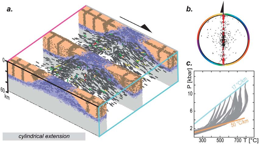
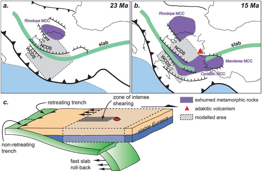
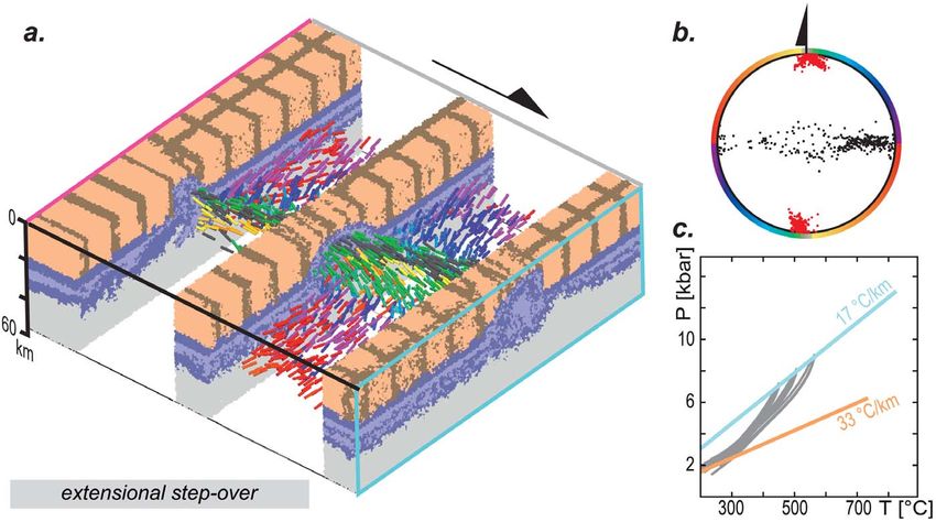
To conclude with a 10 years story:
 Models should not just be a way to reproduce
 Geochemistry 3 geologist concept
 SHAPES OF MCCs at the 10.102
 L. Jolivet et al. / Tectonophysics 659 (2015) 166–182

 end
 Geophysics
 ofInternal
 a project.
 Geosystems
 Figure 4. Results for cylindrical extension (Model 1). (a)
 G LE POURHIET ET AL.: 3D
 171

 deformation of the model outlined by cross-sections
 across the material points and by tubes representing the stretching lineation (maximum stretching axis of the finite strain
 tensor). The tubes are colored by their strike with color scale represented in b. where gray indicates when the lineation is
 Jolivetofettheal.
 aligned with the direction of stretching imposed at the boundary of the model. (b) Stereo-plot representation 2004
 lineation (red) and the foliation (black) for all the tracers located at less than 8 km depth after 12 Myr of simulation.
 (c) Synthetic P-T path for the same tracers as those represented in the stereo-plot in Figure 4b. Initial and final
 thermal gradient in blue and yellow respectively. The final thermal gradient is constrained assuming the line goes
 through 0! at the surface.

 kinematics lead to the exhumation of deep crustal to the free slip side of the model. This trend is
 material to the surface (blue material in Figures 3a therefore parallel to the stretching direction close to
 and 3c), while the step-over kinematics model the back boundary, whereas it is perpendicular to
 does not (Figure 3b). In the case of cylindrical the stretching direction close to the left hand side
 boundary conditions (Figure 3a), the model pro- boundary. Looking in more detail, one sees that in
 duces one structure, elongated normal to the direc- between the two branches, there are less exhumed
 tion of stretching. In the case of fault propagator rocks and that the strike-slip part appears to be
 kinematics, the initially deep crustal material is elongated further toward the back of the model than
 exhumed along a curvilinear trend which follows the location of the(modified
 A Geological cylindrical partJolivet
 of theetexhumed
 Figure 1. (right)
 the fault propagator and turns to become illustrates
 3D sketch
 structure (Figure
 orthogonalthe stereo-plot 3c).
 conceptual
 from model in 2004
 al. [2004]) illustrates two classes of dom
 projections of the lineation (L) and foliation (S) for the two kinds of do
 dome, constriction is important and the foliation is folded with axis aligned with the direction of
 b-type dome, the foliation is folded with an axis normal to the direction of extension. The a-type do
 drical and cannot be modeled in 2D.

 on the impact of 3D boundary conditions on their 2.2. Treatment of the Rheolo
 resulting shape, the model design accounts for most
 [9] At the scale of these model
 First 3D models of of the factors that are known to favor the occur-
 in any given volume has no reas
 rence of MCCs. This includes an initially thickened
 metamorphic core complex pure quartz, pure olivine or plagi
 crust of 50 km [Buck, 1991; Gaudemer et al., 1988;
 be influenced by the layering of
 indicates A types occur Block and Royden, 1990] and an initial thermal
 anisotropy, structural softening an
 gradient which is set to 17.5! C/km. We note that
 in strike slip settings to small scale boudinage and foldi
 this gradient yields a Moho temperature of 875! C,
 is not yet possible to account for al
 which is higher than the 800! C limit proposed by
 in crustal or lithospheric scale m
 Tirel et al. [2008]. At asthenospheric depth, the
 Le Pourhiet et al. 2012 initial
archipelago showing the main metamorphic core complexes and plutons, as well as kinematic indicators. After Gautiertemperature is clamped
 and Brun (1994a,b),
 !
 Huet et al. not to exceed 1300 C
 (Figure
 rasemann et al. (2012), Augier et al. (2015). NCDS: North Cycladic Detachment System. WCDS: West Cycladic 2). The
 Detachment crust itself consists of two layers of
 System.
 25 km each. At a given temperature, the top layer
 Figure 5. Results for extensional step over (Model 2), legend is the same as for Figure 4.
 (brown shades, Figure 2) is mechanically stronger
ay to the Rhodope shows at first order this during a rather short period between ~17 Ma and 8 Ma, which approx-
 than the lower one (blue shades, Figure 2), impos- 6 of 17
agmatic products with time (Jolivet and imately covers the same period as the formation of high-temperature a-
 3). However, the picture is more complex
 ing a step in the strength profile at the interface
 type domes and the fast rotation of the external Hellenides.

They should be used to drive future field/geophysical campaign
 L. Jolivet et al. / Tectonophysics 659 (2015) 166–182 171

 Figure 4. Results for cylindrical extension (Model 1). (a) Internal deformation of the model outlined by cross-sections
 Jolivet
 across the material points and by tubes et al.
 representing the2015
 stretching lineation (maximum stretching axis of the finite strain
 tensor). The tubes are colored by their strike with color scale represented in b. where gray indicates when the lineation is
 Jolivet et al. 2021
 aligned with the direction of stretching imposed at the boundary of the model. (b) Stereo-plot representation of the
 lineation (red) and the foliation (black) for all the tracers located at less than 8 km depth after 12 Myr of simulation.
 (c) Synthetic P-T path for the same tracers as those represented in the stereo-plot in Figure 4b. Initial and final
 thermal gradient in blue and yellow respectively. The final thermal gradient is constrained assuming the line goes
 through 0! at the surface.

 kinematics lead to the exhumation of deep crustal to the free slip side of the model. This trend is
 material to the surface (blue material in Figures 3a therefore parallel to the stretching direction close to
 and 3c), while the step-over kinematics model the back boundary, whereas it is perpendicular to
 does not (Figure 3b). In the case of cylindrical the stretching direction close to the left hand side
 boundary conditions (Figure 3a), the model pro- boundary. Looking in more detail, one sees that in
 duces one structure, elongated normal to the direc- between the two branches, there are less exhumed
 tion of stretching. In the case of fault propagator rocks and that the strike-slip part appears to be
 kinematics, the initially deep crustal material is elongated further toward the back of the model than
 Geologist
 exhumed alongnot aconvinced by which
 curvilinear trend the model
 follows acquire
 the location of the cylindricalGeologist
 part of the exhumed
 now convinced by the model draw a
 the fault propagator and turns to become orthogonal structure (Figure 3c).
 new data strike slip fault

 archipelago showing the main metamorphic core complexes and plutons, as well as kinematic indicators. After Gautier and Brun (1994a,b), Huet et al.
Grasemann et al. (2012), Augier et al. (2015). NCDS: North Cycladic Detachment System. WCDS: West Cycladic Detachment System.

ay to the Rhodope shows at first
 Figure Resultsduring
 order5.this a rather short
 for extensional step period between
 over (Model 2), ~17 Maisand
 legend the8same
 Ma, which
 as for approx-
 Figure 4.
agmatic products with time (Jolivet and imately covers the same period as the formation of high-temperature a-

 We need to generalise this type of interactions
13). However, the picture is more complex
 he nature of magmatism changes through
 type domes and the fast rotation of the external Hellenides.
 This short review of the geological context of the Aegean domain
 6 of 17