LAND VALUE DETERMINATIONS & TAX MAPS - State Tax Commission - Published March 2014
←
→
Page content transcription
If your browser does not render page correctly, please read the page content below
State Tax Commission

LAND VALUE DETERMINATIONS
        & TAX MAPS

          Published March 2014

                     -1-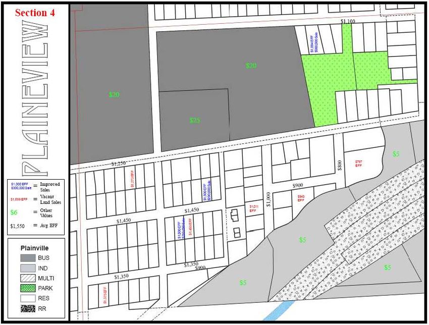
1. OVERVIEW
An assessor is responsible for estimating a land value for every taxable parcel of
property which is valued using the cost approach. Similarly, County equalization
departments must also establish land values to appraise parcels included in
equalization appraisal studies. In establishing land values, you must consider
the general forces (economic, social, environmental, and governmental – zoning
and deed restrictions) that affect the parcels’ value as well as the parcels
physical characteristics. These characteristics include location, size, view,
frontage on a lake or river, topography, shape, existing vegetation, soil (whether
the soil perks, etc.), available utilities, and unusual site preparation costs.

Several methods are available for the land valuation process, including the sales
comparison, allocation, extraction, and subdivision development methods, as
well as several income capitalization techniques. Land values should generally
be applied as calculated and an assessor or equalization director should be
prepared to explain any departures from the calculated land values. It is very
important to keep land values and supporting documentation related to the
development of land values up to date annually.

   2. LAND VALUE DEVELOPMENT METHODS
Sales Comparison Method

Using the sales comparison method, information regarding sales of similar
vacant land is collected, verified, analyzed, and adjusted to give an indication of
value of the property being appraised. The first step in this process is the
collection of vacant land sales data. Verification of sales information is essential
before recording the information on maps or in a spreadsheet format for analysis
as part of the mass appraisal process (or in a standard adjustment grid in single-
property applications).

In analyzing data, it is important for an assessing officer to compare the
characteristics of sold parcels such as location, highest and best use, size, etc.
In mass appraisal situations, this allows the vacant land sales to be grouped
based on similar characteristics and the assessing officer may then assign land
values derived from the grouping to subject properties sharing similar
characteristics with the group.

An important part of the analysis is the use of an appropriate unit of comparison.
The square foot is the most widely used unit of comparison for land valuation.
Because it is an area measurement, it considers all the land in a parcel and can
be used to value any and all types of land. The square foot, as a unit of
comparison, is especially adapted for valuing parcels with irregular shapes. The
square foot is also most commonly used for commercial and industrial parcels.

                                           -2-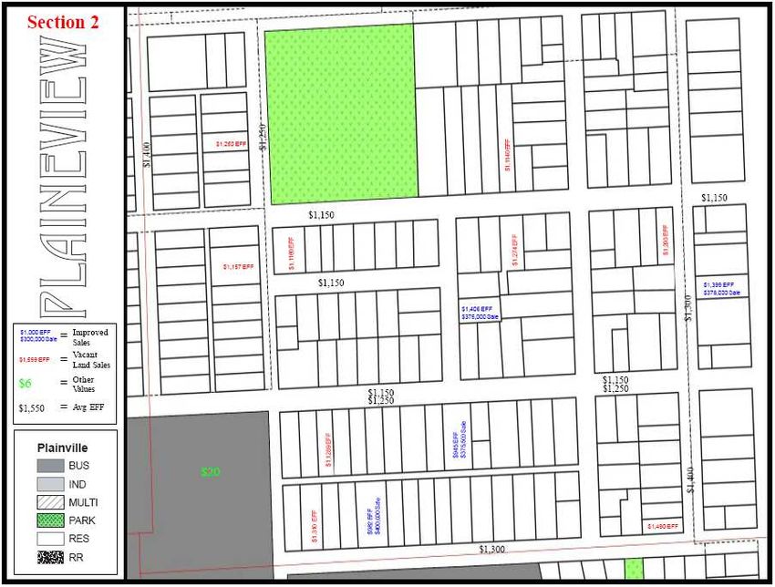
For residential properties, value per front foot, value per square foot, or value per
acre may the best unit of comparison. When using front foot values, it is
necessary to consider a depth factor (the use of depth factors is covered
extensively later in this program). “Frontage” is the lineal distance that a lot
(usually referring to an urban or suburban lot) borders on a street or water, and is
typically expressed in feet. Site or lot values are another option for residential
properties, especially in platted subdivisions. Agricultural land is typically valued
on a per acre basis. The acre is used as a unit of comparison when valuing large
land areas (e.g., farms, pastures, timber lands, recreational lands, etc.).

Selecting the proper unit of comparison is important in gaining an understanding
of how the market is behaving. Conversely, selection of an inappropriate unit of
comparison can lead to faulty results. For example, it would generally not be a
good idea to use front foot values to appraise land which has a highest and best
use of agricultural.

In the mass appraisal process, regardless of the unit of comparison selected, you
must also give consideration to adjustments for positive or negative influences in
setting the land value for a parcel. Influences such as corner lots in residential
settings, high traffic volumes (generally a positive influence for commercial
parcels but generally a negative influence for residential parcels), unusual shape,
unusual topography, nearby nuisances, etc. should be given consideration for
possible adjustment. To the extent possible, adjustments should be derived from
the market. For example, the market would likely recognize that a parcel in a
residential area that has an unusual formation of bedrock just beneath the
surface of the land (which would prevent a normal basement from being
constructed) is worth less than normal for the neighborhood. In such a case, an
assessing officer should determine an appropriate negative adjustment from
available sales information and apply that adjustment to the neighborhood’s front
foot rate (or square foot rate or site value) for the affected parcel.

Regardless of the unit of comparison that is selected for use, it is important to
note that land lying under a public road right-of-way is exempt and should
not be considered in a parcel’s area. For instance, in determining a parcel’s
value per acre the area under a public road right-of-way is not to be included in
the parcel’s area.

A table is provided below containing vacant land sales information compiled in a
mass appraisal situation. The information shown has been collected, verified,
analyzed, and sorted by surface area (size). In this case, the selected unit of
comparison is value per square foot. This information has been developed to the
point where a conclusion of value could easily be drawn and then applied to a
group of subject properties with a highest and best use of office, a land area of
roughly 90,000 to 110,000 square feet, and a good location in the same
assessment unit and local school district in which the vacant land sales occurred.
Where possible, vacant land sales information should be developed and

                                            -3-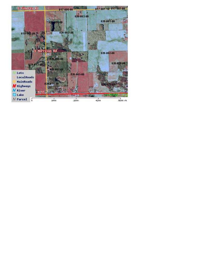
maintained by category of property to be appraised. (In practice the table would
likely contain additional information such as parcel number, grantor, grantee,
liber and page, adjusted sale price, etc.).

                              AREA     SALE PRICE
    SALE         SALE       (SQUARE    PER SQUARE
    DATE        PRICE         FEET)       FOOT              COMMENTS
                                                         Good Location/Future
  1/27/2012    $363,700      88,712         $4.10            Office Site
                                                         Good Location/Future
  10/3/2011    $373,600      90,019         $4.15            Office Site
                                                         Good Location/Future
  2/10/2012    $370,000      91,814         $4.03            Office Site
                                                         Good Location/Future
  8/15/2011    $405,000     100,988         $4.01            Office Site
                                                         Good Location/Future
  12/8/2011    $412,900     101,954         $4.05            Office Site
                                                         Good Location/Future
 11/22/2011    $417,700     108,490         $3.85            Office Site
                                                         Good Location/Future
 10/14/2011    $424,100     111,598         $3.80            Office Site
                                                         Good Location/Future
  5/14/2011    $428,400     113,944         $3.76            Office Site

The information provided above is uniform and logical in nature. In a real world
setting, such a high degree of uniformity and logic is rare. An assessing officer
establishing land values often must deal with difficult or confusing sales
information. It can be common for sales information to contain outliers, which are
values that lie outside the range of values formed by the majority of other sales.
Another common problem is for the sales information to appear not to lead to a
logical conclusion. Or it may be that there is a lack of sales information.
Assessing officers must deal with all of these difficult situations when valuing
land.

                                          -4-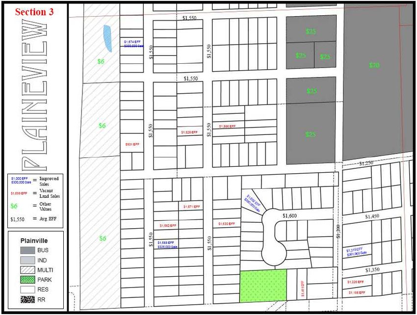
The chart from above has been reproduced with the addition of two outlier sales
shown in strikethrough.

                               AREA      SALE PRICE
     SALE          SALE      (SQUARE     PER SQUARE
     DATE         PRICE        FEET)        FOOT              COMMENTS
                                                           Good Location/Future
   1/27/2012     $363,700      88,712        $4.10             Office Site
                                                           Good Location/Future
   10/3/2011     $373,600      90,019        $4.15             Office Site
                                                           Good Location/Future
  10/25/2011     $495,700     90, 129        $5.50             Office Site
                                                           Good Location/Future
   2/10/2012     $370,000      91,814        $4.03             Office Site
                                                           Good Location/Future
   8/15/2011     $405,000     100,988        $4.01             Office Site
                                                           Good Location/Future
   12/8/2011     $412,900     101,954        $4.05             Office Site
                                                           Good Location/Future
   1/30/2012     $303,850     103,000        $2.95             Office Site
                                                           Good Location/Future
  11/22/2011     $417,700     108,490        $3.85             Office Site
                                                           Good Location/Future
  10/14/2011     $424,100     111,598        $3.80             Office Site
                                                           Good Location/Future
   5/14/2011     $428,400     113,944        $3.76             Office Site

These two sales are considered outliers because their sale prices per square foot
lie well outside the range of values formed by the other sales information. Under
these circumstances, use of the outlier sales information may lead to faulty
results. Often there will be a reason for the divergent sale price. If additional
investigation showed that the buyer and seller involved in the sale for $2.95 per
square foot were business partners and the reduced price was due to their
business association, it would be appropriate to remove that sale from the
analysis. Generally speaking, unexplained outlier sales should be given little
weight in determining land values. They can remain in the chart but should be
noted as inactive and not used in the analysis. If additional review does not
reveal a valid reason to remove that sale from the analysis, the sale may remain
in the chart, however it should not be given much weight in reaching a land value
conclusion.

The following chart contains residential vacant land sales information. All of the
sales information comes from the same residential subdivision and the same
time period (and assume for this example that the lots all have the same depth).
Looking at this information it would be difficult to determine the proper land value
to use in this subdivision. As an example, the four indicated values for lots having

                                           -5-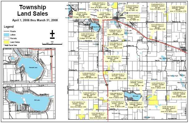
85 feet of frontage are: $547, $550, $625, and $647. Additional analysis is
needed to form a conclusion regarding the appropriate front foot values to use.
                                              SALE PRICE
     SALE          SALE            FRONT      PER FRONT
     DATE         PRICE             FEET        FOOT           COMMENTS
   2/27/2012      $45,000            75          $600         Residential Site
   8/13/2011      $55,000            75          $733         Residential Site
   11/25/2011     $56,000            75          $747         Residential Site
   1/10/2012      $46,400            80          $580         Residential Site
    6/6/2011      $54,000            80          $675         Residential Site
   10/8/2011      $47,000            80          $588         Residential Site
   2/30/2012      $46,500            85          $547         Residential Site
   10/29/2011     $46,750            85          $550         Residential Site
   7/14/2011      $53,125            85          $625         Residential Site
   5/15/2011      $55,000            85          $647         Residential Site

When the assessor does more research, they find that a local school district
boundary cuts through this subdivision. With this additional piece of the puzzle in
place, a definite pattern emerges from the data, as shown below. School district
B is clearly more desirable than school district A and the assessing officer can
use the information below to establish reliable front foot rates for lots in this
subdivision. The important point to remember from this example is that, with
additional analysis, confusing data can be turned into meaningful information.

                                      SALE PRICE
   SALE          SALE       FRONT     PER FRONT
   DATE         PRICE        FEET       FOOT                COMMENTS
                                                        Residential Site/School
 2/27/2012      $45,000       75           $600               District A
                                                       Residential Site/School
 8/13/2011      $55,000       75           $733               District B
                                                       Residential Site/School
 11/25/2011     $56,000       75           $747               District B
                                                        Residential Site/School
 1/10/2012      $46,400       80           $580               District A
                                                       Residential Site/School
  6/6/2011      $54,000       80           $675               District B
                                                        Residential Site/School
 10/8/2011      $47,000       80           $588               District A
                                                        Residential Site/School
 2/30/2012      $46,500       85           $547               District A
                                                        Residential Site/School
 10/29/2011     $46,750       85           $550               District A
                                                       Residential Site/School
 7/14/2011      $53,125       85           $625               District B
                                                       Residential Site/School
 5/15/2011      $55,000       85           $647               District B

                                           -6-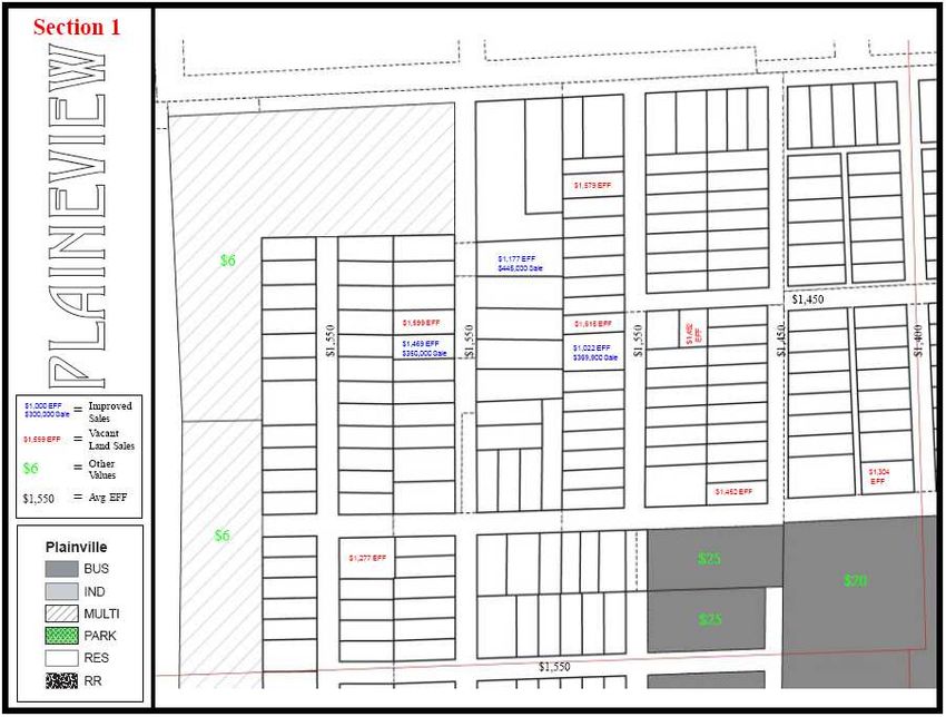
In many situations, an assessing officer setting land values will be faced with a
lack of sales information. For example, an assessor trying to establish land
values for tillable land in his jurisdiction may not have any sales within the entire
Township during the two-year sales study period.               Likewise, a county
equalization department trying to create industrial land values may not have any
industrial vacant sales in the county over the past several years. In difficult
situations like these, land values must still be determined and used.

When there is a lack of sales information, the assessor should use sales outside
the normal time frame of the sales study period, or use sales from outside the
area for which land values are being determined. If sales from outside the
normal time frame of the sales study period are used, adjustment for market
conditions (i.e., a time adjustment) should be made to bring the sales to the
midpoint of the sales study period. If sales from outside the area for which land
values are being determined are used, adjustment for location should be made.

The calculations below demonstrate how to determine an adjustment from
market data for changing market conditions or time:

Original sale price (two years ago):                 $175,500 (A)
Sale price of same property (present time):          $182,000 (B)
Change over two-year period (B ÷ A - 1 = C):     .0370, 3.70% (C)
Percentage change per year (3.70% ÷ 2 years = D):       1.85% (D)

The analysis above is called a “paired sales analysis”. A paired sales analysis is
a technique to identify and measure adjustments to sales prices or rents of
comparable properties. In order to apply this technique you need to use
properties that are identical or as nearly identical as possible. A paired sales
analysis will help you identify and isolate the effect of a single variable on the
value of a property, for example time.

The example above indicates a 1.85% increase in market value per year for the
subject property (this assumes no physical changes to the property, etc. over that
time). Using paired-sales analyses like this, an assessor can determine an
appropriate time adjustment and then apply that time adjustment to older sales to
supplement existing sales information and determine land values for an area. It
should be kept in mind that a single paired sales analysis is generally not
considered sufficient to justify the adjustment of older sales information to the
mid point of the current sales study period.

The following demonstrates how to make an adjustment for location from market
evidence. Sale 1, for $27,000, is a vacant lot located in subdivision A which has
no other vacant land sales. The assessor is trying to establish land values for
subdivision A. Sale 2, for $25,000, is a vacant lot located in subdivision B which
is similar to subdivision A. These two vacant lots are similar in all respects

                                            -7-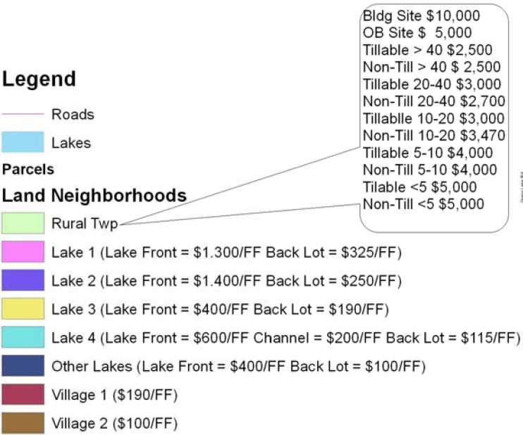
except for location. The calculations below demonstrate how to determine an
adjustment from market data for location:

Sale 1:                                                   $27,000 (A)
Sale 2:                                                   $25,000 (B)
Difference in value due to location (A ÷ B – 1 = C): .080 or 8.0% (C)

This paired-sales analysis indicates that subdivision A is 8.0 % superior in
location to subdivision B (i.e., this indicates that the assessor should use a
multiplier of 1.080 to adjust vacant land sales from subdivision B to arrive at a
land value conclusion for subdivision A). Using paired-sales analyses like this,
an assessing officer can determine an appropriate location adjustment and then
apply that adjustment to sales outside subdivision A to supplement existing sales
information and determine land values for subdivision A. Assessors are
cautioned that a single paired-sales analysis is generally not sufficient to justify
the adjustment of sales outside the area in question for location and that a long
time period on any type of paired sales analysis is not useful; over a long period
trends will tend to be fairly normal looking.

As a last resort, an assessor could consider reviewing “asking prices” to help
establish land values. If an assessor is going to use this method, they need to
understand that actual sale prices are typically a percentage of “asking price”.
For example, an asking price of $119,900 might result in an actual sale price of
$110,000. It is important for an assessor to know their market extremely well
when considering “asking price”. Discussions with knowledgeable sources,
realtors, and fee appraisers may be used to support land value conclusions
drawn by an assessor.

Practical Exercise for Time Adjustments:

The first step in determining a time adjustment is to locate parcels that are twice
sold i.e.: those sold twice in a given time period. It is important to verify that
there were no physical changes to the parcel between the sales. Divide the most
recent sale price by the original sale price to determine the overall percentage of
change. Finally, divide the overall percentage of change by the number of time
periods between the two sales to determine the percentage change per month or
year.

Below are is an example of twice-sold parcels. Fill in the blanks.
Original sale price (Sept 1, 2004):                                   $225,000 (A)
Sale price of same property (April 1, 2009):                          $305,000 (B)
Percentage change in value between sales (B ÷ A – 1 = C):                      (C)
Percentage change in value per month (55 months):                              (D)

Original sale price (December 10, 2006):                              $325,000 (A)
Sale price of same property (March 11, 2008):                         $355,000 (B)

                                           -8-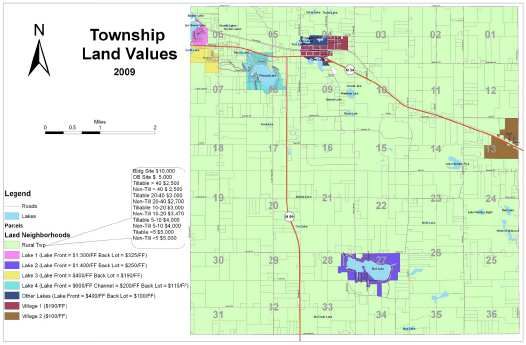
Percentage change in value between sales (B ÷ A – 1 = C):                   (C)
Percentage change in value per month:                                       (D)

The paired-sales analyses above are of commercial parcels in a given assessing
unit. Would it be appropriate to use a time adjustment determined from the
above analyses for industrial parcels within that same assessment unit? Why or
why not?

The paired-sales analyses above are from the time period September 2004 to
April 2009. Would it be appropriate to apply a time adjustment determined from
the analyses above to a sale that occurred in March of 2009 to bring that sale
forward to April of 2012? Why or why not?

Time Adjustment Answers

Below are two twice-sold parcels which have been discovered through research.
Fill in the blanks.

Original sale price (September 1, 2004):                 $225,000 (A)
Sale price of same property (April 1, 2009):             $305,000 (B)
Percentage change in value between sales (B ÷ A = C): 1.356, 35.6%(C)
Percentage change in value per month:                        0.65%(D)

Original sale price (December 10, 2006):                   $325,000 (A)
Sale price of same property (March 11, 2008):              $355,000 (B)
Percentage change in value between sales (B ÷ A = C):    1.092, 9.2%(C)
Percentage change in value per month:                         0.61%(D)

The paired-sales analyses above are of commercial parcels in a given assessing
unit. Would it be appropriate to use a time adjustment determined from the
above analyses for industrial parcels within that same assessment unit? Why or
why not?

No. Market conditions typically affect industrial properties differently than
commercial properties. It would not be appropriate to use a time adjustment
determined above from commercial parcels for industrial parcels within that same
assessment unit.

The paired-sales analyses above are from the time period September 2004 to
April 2009. Would it be appropriate to apply a time adjustment determined from
the analyses above to a sale that occurred in March of 2009 to bring that sale
forward to April of 2012? Why or why not?

                                         -9-
No. Market conditions between April of 2009 and April of 2012 may well have
been different than the market conditions covered by the paired-sales analyses
(the last sale in the analyses occurred in April of 2009). It would not be
appropriate to apply a time adjustment determined above to a sale that occurred
in March of 2009 to bring that sale forward to April of 2012 without additional
support of some kind from the market or from market participants.
Example Land Value Analysis
A land value analysis grid and a plat map follow as part of an example land value
analysis using the sales comparison approach. In this analysis, several of the
lots in the plat have sold and an appropriate analysis (the grid) and resulting
conclusions are provided to show how to conduct a vacant land value analysis
for a neighborhood.
EXAMPLE LAND VALUE ANALYSIS GRID
Effective
Sale Sale Front Square Front
Lot Date Price Feet SP/FF Feet SP/SF Feet SP/EFF
1 11-11 $10,000 100 $100 15,000 $0.67 100 $100
6 2-12 $9,975 100 $100 15,000 $0.67 100 $100
11 5-11 $11,000 97 $113 13,580 $0.81 97 $113
12 8-11 $10,900 97 $112 13,580 $0.80 97 $112
24 9-11 $10,300 92 $112 13,800 $0.75 92 $112
31 7-11 $10,500 96 $112 12,468 $0.84 94 $112
37 8-11 $10,750 85 $124 13,983 $0.77 87 $119
41 1-12 $12,600 95 $134 17,815 $0.71 94 $134
45 4-11 $10,000 100 $99 15,204 $0.66 101 $99
46 5-11 $10,250 100 $101 15,204 $0.67 101 $101
If the front of a lot is a different size than the rear, the formula for determining the frontage is as
follows: ((2 X front feet) + rear feet) ÷ 3. In this case, the front of the lot is 96 feet and the rear of
the lot is 90 feet. The calculation for the frontage to use in valuing the parcel is as follows: ((2 X
96 feet) + 90 feet) ÷ 3 = 94 feet. The frontages of other lots (37, 41, 45, and 46) in this example
are determined in this manner as well.
Lots 1, 6, 45, and 46 are on the exterior of the plat and border on major roads
(with higher speeds, greater traffic counts, etc.). The lower values of these lots
reflect this negative influence. Lots 1, 6, 45, and 46 all have lower values per
front foot and per effective front foot. The use of a site or lot value would work
well for these as well. The remaining lots are all interior lots within the
subdivision. The use of lot or site values for these lots would be less than ideal.
Also, the sale price per front foot for these lots is less consistent. Using the sale
price per effective front foot, however, yields consistent results for all the lots in
the subdivision, with the exception of lot 24 which appears to be an outlier and
should carry little weight in the analysis. Based on this analysis, a value of $100
per effective front foot appears appropriate for lots bordering on major roads and
a value of $118 per effective front foot appears to be indicated for interior lots
- 10 -within the subdivision. Alternatively, a rate of $118 per effective front foot could
be used for all the lots with a negative location adjustment (of about $18 per
effective front foot) used to value lots on major roads).
- 11 -ALLOCATION METHOD
When limited sales data are available in a given neighborhood or area, it is
sometimes necessary to use alternative methods of land valuation. In the
allocation method, the assessor first determines a typical ratio of land value to
total property value (or building value) for the specific type of property being
appraised and then infers land value for the subject property or properties by
applying that ratio. This method can be used when sales of vacant land are
scarce (or non-existent) in a given area, but where there have recently been
sales of improved properties and is especially applicable in residential appraisal
situations.
This method is generally considered less reliable than the sales comparison
method. However in completely developed neighborhoods it can provide a fairly
good indication of value if a good analysis is conducted and outliers are reviewed
and investigated.
If an assessor needs to determine land values for residential lots in a new
subdivision A, which has not had any vacant land sales activity, and the assessor
has a more established subdivision B, which is somewhat similar to subdivision A
and has sufficient sales of both vacant and improved land; using the allocation
method, the assessor would first analyze vacant land sales in subdivision B and
determine their relationship to the improved sales in subdivision B.
Based on that analysis, if the assessor could conclude that land values in
subdivision B are typically around 25% of the sale price of improved properties,
then a ratio of 25% could be used to assign land values to lots in subdivision A
based on improved property sales in subdivision A. As an example, if an
improved sale occurred in subdivision A with a sale price of $350,000, the
assessor would multiply that sale price by 25% ($350,000 x 0.25), giving an
indicated land value of $87,500.
- 12 -Allocation Method Example: In this example, there is sufficient sales
information available for improved parcels within neighborhood “A” but few sales
of vacant land. Both vacant and improved sales in a similar neighborhood B are
available:
Vacant / Sale Indicated Ratio LV Ratio LV
Improved Address Price LV to Prop to Bldg
Vacant 8730 Clarion $77,000
Vacant 8700 Clarion $73,000
Indicated LV-> $75,000
Improved 8719 Clarion $376,000 20% 1 to 5 1 to 4
Vacant 8829 Bonaventure $58,000
Vacant 8718 Bonaventure $63,000
Indicated LV-> $60,000
Improved 8803 Bonaventure $310,000 19% 1 to 5 1 to 4
Vacant 8601 Bonaventure $68,000
Vacant 8665 Bonaventure $72,500
Indicated LV-> $70,000
Improved 8713 Bonaventure $340,000 21% 1 to 5 1 to 4
Conclusion: Land Value to Prop. or Bldg. Value Ratio 1 to 5 1 to 4
NEIGHBORHOOD “A” VALUES – Based on a Land to Property Value Ratio of 1
to 5 (20% of Property Price or Value)
Sale Price or Indicated Building
Parcel Number Address Property Value Land Value Value
4716-19-201-056 8873 Vista $412,000 $82,400 $329,600
4716-19-201-060 8969 Vista $390,000 $78,000 $312,000
4716-19-201-068 9439 Wendover $350,000 $70,000 $280,000
4716-19-201-074 9452 Wendover $450,000 $90,000 $360,000
4716-19-201-075 9436 Wendover $335,000 $67,000 $268,000
4716-19-201-077 9404 Wendover $400,000 $80,000 $320,000
4716-19-201-081 8878 Vista $362,000 $72,400 $289,600
The chart above shows an indicated site value based on a land to property value
ratio of 1 to 5 and or a land to building value ratio of 1 to 4. In analyzing a sale
using this data, you would use the land to property ratio of 1 to 5 (20%) against
the sale price to estimate a land value. In conducting a cost appraisal, you would
determine the building value (RCNLD), and then use the land to building ratio 1
to 4 (25%) to estimate the land value.
- 13 -EXTRACTION METHOD
The extraction method is another alternative method of land valuation which can
be used when there is insufficient vacant land sales information. This method is
considered one of the least reliable methods due to the difficulty of measuring
accrued depreciation. It does however work fairly well on relatively new
structures that have recently sold as long as a proper Economic Condition Factor
has been calculated.
In this method, an estimate of the depreciated cost of improvements is
subtracted from the sale price of an improved property leaving an estimate of the
value of the land. For example, an improved property that sold for $375,000 with
an estimated depreciated cost of improvements of $262,500 would suggest a
land value of $112,500 ($375,000 - $262,500 = $112,500).
SUBDIVISION DEVELOPMENT METHOD
This method is often used to value land in transition between uses, such as from
agricultural use to a residential or commercial use. Under this method the
assessor would use highest and best use. For example: assume the highest and
- 14 -best use for the parcel is for development into a residential subdivision. The
assessor first would estimate the costs associated with developing the parcel into
a subdivision and then subtracts those costs from the anticipated sale prices of
the developed sites. Because the subdivision development method uses many
items that are difficult to accurately measure, use of method should be limited to
cases where there are an insufficient number of sales of similar parcels available
for development. A primary consideration in using this method is that the land
must be ripe for development and either zoning permits this use or there is a
reasonable probability of a change in zoning to allow this use.
Subdivision Development Method Example: A 20-acre parcel is zoned for
single-family residences which is also the highest and best use of the property.
Assuming the parcel can be developed into four lots to the acre, including
streets, the first consideration is supply and demand as well as purchasing
power. The market indicates a value of $40,000 per lot, or $3,200,000, when the
parcel has been completely developed (4 lots per acre X 20 acres = 80 lots; 80
lots X $40,000 per lot = $3,200,000). Research then needs to be done into
anticipated site development costs, including overhead, sales expenses, profit,
and interest during development.
Example:
• Site development (streets, sewers, water service, site preparation,
planning), 25 %
• Overhead and sales expenses (commissions, title work, advertising,
general office expenses, accounting and legal expenses), 25 %
• Profit and interest cost during development and holding period, 25 %
Based on this information the remaining 25% of lot sales can be attributed to the
contributory value of the raw land. The value of the land under the subdivision
development method is then $800,000 ($3,200,000 total indicated value X 0.25 =
$800,000 land value).
DEPTH FACTORS
A depth factor is used, usually in urban or suburban settings, to adjust land value
for differences in the actual depth of a parcel compared to the standard or typical
depth for an area. A lot that is deeper than the standard depth lot will usually
have more value and a lot that has less depth than the standard lot will usually
have less value. Depth factors allow for a uniform amount per front foot to be
used to value parcels of different depths by adjusting for differences in depth by
converting actual frontage into equivalent front feet. This equivalent frontage,
multiplied by the established front foot value, gives the appraised value of the lot.
Depth factor tables can be used instead of calculating individual depth factors for
each parcel being valued. If a depth factor table is used, the resulting values
should be checked against market information to ensure that the table is
- 15 -appropriate for the area being valued. When using a depth factor table (reprinted
from the STC manual), it should be kept in mind that a given depth factor table
will not work in all valuation situations.
- 16 -Depth factors account for differences between the lots with a standard depth and
lots with depths that vary from the standard lot depth. A lot is of standard depth
when it has a depth that is common for most other lots in the area. In the
drawing below, lots 5 and 7 do not have standard depths while the remaining lots
do have a standard depth.
5
1 2 3 4 6 8
7
Rose Street
If several of these lots have recently sold, an amount per front foot can be
developed:
Lot Number Sale Price Front Feet (FF) Sale Price Per FF
2 $16,500 80 $206
4 $12,000 60 $200
6 $14,500 70 $207
Indicated Value Per Front Foot: $205
From this information, $205 per front foot is appropriate for lots within this
subdivision and all of the lots that have sold are standard depth lots. If the front
foot rate of $205 is applied to all of these lots, will it be representative of the
market value of each lot? Most people would probably argue that lot 5 should
sell for more per front foot because of the additional depth, and lot 7 should sell
for less. The use of a depth factor will adjust the front foot rate used for the lots
and compensate for the differences in depth.
Using the table above, assume that the standard depth of the lots is 120 feet.
Lot 5 is 140 feet deep and lot 7 is 60 feet deep. Both lots have 60 feet of
frontage. Using the depth factor table provided, locate the column for standard
depth of lot, 120 feet. Lot 5 is 140 feet deep, so go to the left hand column which
has a heading of “Actual Depth of Lot”; following across to the right to the column
120 feet, the depth factor is 108. Do the same exercise for the 60 feet actual
depth for lot 7, the depth factor is 71. The next step is to apply the depth factor
to the actual front feet and then value the lots using the calculated front foot rate:
- 17 -Lot 5 actual frontage = 60 X 108% = 64.8; 64.8 X $205 = $13,284 or $13,300
rounded
Lot 7 actual frontage = 60 X 71% = 42.6; 42.6 X $205 = $8,733 or $8,700
rounded
Formula used to calculate the depth factors:
.
Depth factor = √actual lot depth ÷ standard lot depth
Example: 150 feet actual lot depth ÷ 120 feet standard lot depth = 1.25,
1.25 = 1.12
3. LAND VALUE MAPS
Land value maps are a graphical presentation of land values for an entire
assessment unit (i.e., an entire City or Township). A graphical display of land
values enables the assessor to explain and defend the results of his or her land
value analyses to taxpayers. Constructing land value maps also helps keep the
assessor informed of land value changes or patterns in the assessment
jurisdiction. Significant information which might not otherwise be noticed often
becomes apparent when land value information is presented graphically.
MCL 211.10e requires that assessors maintain land value maps consistent with
the standards provided in the State Tax Commission’s Assessor’s Manual. Land
value maps are defined in the Assessor’s Manual as “maps on which are
recorded the front or square foot value of platted property and the square foot or
per acre value of acreage property.” A good set of land value maps will contain
both, the value conclusions for land used by the assessor to determine
assessments, and the vacant land sales information used by the assessor to
reach those conclusions. This may take the form of two sets of maps (one with
sales information and the other with the assessor’s value conclusions). It is a
good practice to have individual land value maps, or color coded at a minimum,
for different classes of property such as agricultural, residential, commercial, etc.
To set up a land value map system, you have to put together a set of maps for
the entire assessing district. Types of maps that can be used include, but are not
limited to, copies of tax maps; copies of recorded plats of subdivisions; City,
Township, and County street maps; aerial photographs with map overlays; and
zoning and land use maps. Maps need to be at a useful scale. Once a set of
maps has been put together, known vacant land sales information which has
been verified should be added to the maps. The sales information should be put
on the map in an appropriate unit of comparison for the type of property involved.
The land value conclusions of the assessor should also be added to the maps.
This information will enable a property owner to see how his or her land has been
valued as well as the supporting information behind that valuation. This
- 18 -graphical presentation can be extremely helpful in explaining and defending
assessments.
TYPES OF LAND VALUE MAPS
Land value maps can be prepared in different formats depending on the
circumstances. A land value map for an urban area will be different from a land
value map for a rural area. While the land value maps presented here were
produced through the use of computers, it is not necessary to have that level of
technology to produce an acceptable land value map; acceptable land value
maps can also be produced by hand.
The following map shows vacant land sales information. The map is for a rural
Township. Portions of the map have also been reproduced below the map to
make them large enough to be read. Map should be printed in a scale that would
allow the map to be legible. The sold parcels have been highlighted on the map
and details regarding the land sale have been noted. The parcel number, the
date of sale, the total sale price, and the sale price expressed in terms of a unit of
comparison have all been noted for each sale on the map. This information is
useful in establishing land values to be applied by the assessor.
- 19 -The map show above is one half of what is considered to be sound assessing
practices with regard to land value maps. The other half is a map showing the
land value conclusions used by the assessor to determine assessments. This
map is for the same rural Township pictured in the map on the previous page but
shows the value conclusions.
Note the number of land value neighborhoods for this Township. The Rural Township
neighborhood uses a rate for a building site and an outbuilding site as well as rates for t
- 20 -The legend from this map has been enlarged so that you can see the land value
neighborhoods and the rates used for each neighborhood. Neighborhoods are
broken out for tillable and non-tillable acreages, for lake areas and for the
Villages within the Township (i.e., more dense developments). Any commercial
or industrial areas should also be included. In many cases, this type of land
value neighborhood breakdown will be sufficient. For a rural Township it is not
usually necessary to have a significant number of land value neighborhoods.
Often in cases like this, ‘less is more’ when it comes to land value analysis.
Having too many land value neighborhoods can result in land value analysis
complications due to a lack of sales information in each neighborhood, etc.
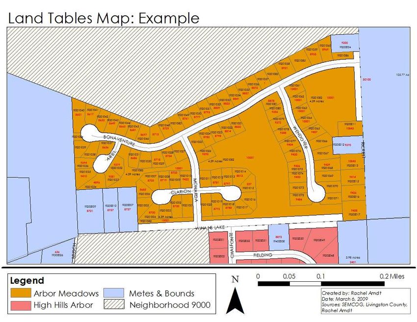
EXAMPLE LAND VALUE MAPS AND LAND VALUE DATA
Example land value maps and land value data are presented on the following
pages and includes: Valuation of residential land in a hypothetical city; land sales
information that has been verified, collected, and converted to equivalent front
foot rates; maps produced using the land sales information and; application of
the allocation method as support for land value conclusions reached by the City.
In Anywhere, Michigan, residential lots are valued on an equivalent front foot
basis. Under this system, a lot that is deeper than the standard lot is assigned
an increased value and a lot that has less depth than the standard lot is assigned
a reduced value through the use of depth factors. The standard depth of a
residential lot in the City of Anywhere is 120 feet. The depth factor table from the
Assessor’s Manual, is used in this example to adjust for differences in the depths
of the different lots. The goal of the example situation is to arrive at an accurate
front foot rate.
- 21 -The table provided shows residential vacant land sales in the City from the two-
year equalization study period. This represents all the verified residential vacant
land sales activity in the City over this period. The table also shows the
equivalent frontages for the sale parcels. Equivalent frontages have been
divided into the sale prices to determine the sale prices per equivalent front foot.
This provides indications of appropriate front foot rates for residential lots.
RESIDENTIAL VACANT LAND SALES FOR ANYWHERE, MICHIGAN
Sale
Price
Parcel Property Sale Front Depth per
Number Class * Sale Date Price Feet Depth Factor EFF EFF
15-15-127-015 401 2/18/2011 $95,000 55.00 140.00 1.08 59.40 $1,599
15-15-128-016 401 11/22/2010 $75,900 44.50 140.00 1.08 48.06 $1,579
15-15-128-024 401 4/14/2011 $75,000 43.00 140.00 1.08 46.44 $1,615
15-15-130-002 401 4/27/2010 $80,000 65.00 86.00 0.85 55.25 $1,448
15-15-130-019 401 5/30/2010 $69,000 44.00 140.00 1.08 47.52 $1,452
15-15-132-012 401 6/6/2011 $120,000 92.10 124.00 1.02 93.94 $1,277
15-15-176-006 401 7/12/2011 $95,000 100.00 124.00 1.02 102.00 $931
15-15-177-012 401 12/20/2010 $82,500 50.00 140.00 1.08 54.00 $1,528
15-15-178-027 401 5/13/2010 $75,500 40.00 170.00 1.19 47.60 $1,586
15-15-181-005 401 3/10/2011 $82,000 50.00 132.00 1.05 52.50 $1,562
15-15-181-016 401 9/12/2010 $82,500 50.00 132.00 1.05 52.50 $1,571
15-15-182-005 401 5/5/2010 $84,900 50.00 148.00 1.11 55.50 $1,530
15-15-182-033 401 9/28/2011 $79,000 50.00 150.00 1.12 56.00 $1,411
15-15-202-014 401 10/24/2010 $65,000 50.00 130.00 1.04 52.00 $1,250
15-15-203-011 401 7/17/2010 $79,000 45.00 279.00 1.52 68.40 $1,155
15-15-204-015 401 3/13/2012 $95,000 72.85 120.00 1.00 72.85 $1,304
15-15-205-011 401 11/22/2011 $125,000 100.00 139.00 1.08 108.00 $1,157
15-15-206-010 401 10/30/2011 $105,000 90.50 120.00 1.00 90.50 $1,160
15-15-208-003 401 12/9/2011 $69,000 45.00 171.00 1.19 53.55 $1,289
15-15-208-018 401 9/21/2011 $95,000 60.96 171.00 1.19 72.54 $1,310
15-15-229-002 401 2/2/2012 $82,500 59.42 143.00 1.09 64.77 $1,274
15-15-230-004 401 8/17/2011 $69,500 48.00 149.00 1.11 53.28 $1,304
15-15-233-013 401 1/15/2012 $59,000 40.00 118.00 0.99 39.60 $1,490
15-15-254-016 401 1/11/2012 $64,900 51.00 120.00 1.00 51.00 $1,273
15-15-256-003 401 7/15/2011 $84,500 60.00 157.00 1.15 68.40 $1,235
15-15-258-003 401 11/13/2010 $72,500 50.00 120.00 1.00 50.00 $1,450
15-15-259-009 401 8/17/2011 $69,000 75.00 100.00 0.91 68.25 $1,011
15-15-260-002 401 1/11/2011 $82,500 60.00 159.00 1.15 69.00 $1,196
15-15-261-015 401 4/3/2011 $72,900 53.00 120.00 1.00 53.00 $1,375
15-15-279-003 401 11/29/2010 $50,000 50.00 133.00 1.05 52.50 $952
15-15-280-002 401 2/22/2012 $185,000 180.00 200.00 1.29 232.20 $797
*401 = Residential Classification
*EFF = Equivalent Front Foot
- 22 -Note: Using the preceding vacant land sales information, land value maps
showing both prices and values have been created. All the vacant land sales
have been plotted on four maps as shown below in the enlarged map area inset.
For each sale, the verified sale price per effective front foot is shown. Also
shown is the rate per effective front foot derived using the allocation method to
support the vacant land sales information. Finally, value conclusions reached by
the assessor to value the lots are shown in the road right-of-way areas. An
overall City zoning map for the City of Anywhere is shown with additional maps
showing smaller areas and the various land sales (in value per equivalent front
foot) and the concluded land values for each street.
Enlarged Map Area
Sale Price per
Effective Front Foot
Front Foot Value Indication from the
Allocation Method
Front Foot Value Conclusion
- 23 -- 24 -
- 25 -
- 26 -
- 27 -
- 28 -
In reviewing the vacant land sales information, it was determined that the amount
of vacant sales data was not ideal and that this lack of sales data would be a
weakness in establishing residential land values in some neighborhoods in the
City. It was decided to use the allocation method to support the value
conclusions reached by the assessor.

The table below shows an analysis of sales of improved residential properties
paired with sales of residential vacant land to determine the proper allocation.
The analysis indicates that land value is approximately 25% of the total value of
improved parcels, based on sales that have occurred in the City. That ratio was
applied to a number of (verified) improved sales in town. The sale prices of the
improved sales were also posted to the land value maps along with the
equivalent front foot value associated with each improved sale. The equivalent
front foot value was calculated by taking 25% of those sale prices and dividing
the result by the equivalent front footage of each sold parcel. In this case, the
resulting allocated land values were converted to equivalent front foot rates to be
consistent with the unit of comparison used in other neighborhoods throughout
the City. (See the maps on the preceding pages.)

                    CITY OF ANYWHERE, MICHIGAN
               LAND VALUATION BY ALLOCATION METHOD
                                  UNIMPROVED (VACANT)                     Ratio of
       IMPROVED PARCELS                 PARCELS                         Unimproved
                                                                          (Vacant)
                             Verified                      Verified     Sale Price to
    Parcel                     Sale          Parcel          Sale        Improved
   Number       Sale Date      Price        Number           Price       Sale Price
15-15-127-018   7/31/2011    $350,000    15-15-182-033     $79,000          23%
15-15-128-040   5/17/2010    $445,000    15-15-132-012     $120,000         27%
15-15-128-048   4/25/2010    $369,900    15-15-176-006     $95,000          26%
15-15-135-003   3/30/2012    $300,000    15-15-128-024     $75,000          25%
15-15-177-003   5/19/2011    $324,900    15-15-130-002     $80,000          25%
15-15-181-007   8/31/2011    $325,000    15-15-181-016     $82,500          25%
15-15-204-010    7/1/2010    $265,000    15-15-208-003     $69,000          26%
15-15-229-016   8/11/2010    $375,000    15-15-208-018     $95,000          25%
15-15-255-012   9/16/2010    $290,000    15-15-261-015     $72,900          25%
15-15-256-001   1/30/2012    $361,900    15-15-256-003     $84,500          23%
                TOTALS:     $3,406,700         ---         $852,900         25%

    4. AGRICULTURAL PROPERTY
Every county in Michigan has agricultural land.    The agricultural classification of
property includes a wide variety of uses, which    are considered agricultural use.
Section 211.34c of the General Property Tax         Law provides that “agricultural
operations” means farming in all its branches,     including cultivation of the soil;

                                          - 29 -
growing and harvesting of any agricultural, horticultural, or floricultural
commodity; dairying, raising of livestock, bees, fish, fur-bearing animals, or
poultry; turf and tree farming; and performing any practices on a farm as an
incidental to, or in conjunction with these farming operations.
The method used to appraise any individual parcel of agricultural property will
depend upon the most likely use of the parcel should it be sold. If the most likely
use is as a cash crop farm, then the comparables should be sales of similar cash
crop farms. For cash crop farms where soil productivity has a direct influence on
value, a method known as the equivalent acreage method is commonly used to
determine the value of soil. The equivalent acreage method is an appraisal
technique which utilizes soil types and the productivity of each soil type to
estimate the usual selling price. If the most likely use is a dairy farm, the
comparables should be sales of similar dairy farms. If the most likely use is a
change to commercial use, comparables should be sales of similar parcels being
converted to commercial use.
Public Act 386 of 1976 provides that the value of land subject to a public right of
way shall not be considered when the real property is being assessed. A later
Attorney General Opinion stated “Land over which is located a county drain right
of way is exempt. However, the legislature was careful to extend the exemption
only to surface rights of way. Subsurface drains, or other rights of way, do not
come within the exemption created by 1976 P.A. 386.”
AGRICULTURAL LAND VALUE INFLUENCES
Factors that influence farm land values can be grouped into general and specific
categories. General factors influence the level of land values in a region and will
commonly result in one area being known as a “fruit belt,” while another area will
be known as a “cash crop area.” These factors include such items as:
1. Length of growing season
2. Precipitation
3. Proximity to and type of markets
4. Proximity to and type of transportation
5. Topography
Specific factors influence the land value of a limited parcel within a given region.
Specific factors include such items as:
1. Productivity of the soil
2. Slope
3. Drainage
4. Management practices
5. Parcel size and shape
6. Quality and availability of water supply
- 30 -Among the specific factors, parcel size and shape is sometimes given too little
attention as to its effect on tillage operations. The presence of transverse
ditches, pot holes, and other barriers can seriously reduce the value of otherwise
productive land. The element of water supply should always be considered. Is
there a plentiful supply? Are there restrictions on use? How deep are drilled
wells? Is there an unusual mineral content? Can irrigation water be obtained
from surface sources? Often, the issue is not supply but of quality for a particular
use.
There are various combinations of the factors listed with the result that some
areas may have unusually high land values for growing certain crops but similar
land located elsewhere may exhibit very low land values for other crops. The
first step an appraiser of farm land should take is to become familiar with general
and specific factors which may have a bearing on the appraisal problem. There
is a wealth of data available at various agricultural agencies in each county of the
state.
5. Forest/Timberlands Property
Timberland or forest land typically includes parcels which are stocked with forest
products of merchantable type and size and are not used for suburban or urban
purposes. If you have determined that growing timber or other forest products is
the dominating use of a parcel, the following are general procedures used to
value forest or timberland property.
1. Determine the type or class of land. (Be certain the parcel is properly
classified.)
2. Determine the type and extent of cover.
3. Determine the present and anticipated utilization of the parcel.
4. Estimate property values by comparing with similar properties. Any of the
methods described later in this chapter may be used providing you
correlate the method with the local market and apply the method in a
uniform manner.
The forest land schedule must closely parallel the local forest land market at the
time the schedule is used. Forest land values vary from region to region and can
change over time. Land value schedules should be constructed from a
background of experience in the sale or purchase of similar lands. There should
be a substantial number of transactions to analyze. Lacking a good market for
forest land, a preliminary schedule may be devised by careful analysis of the
factors affecting land value. These schedules should then be carefully tested
against a selected number of properties. If these properties sell at or near the
schedule values, the schedules may be applied with a certain amount of
confidence. The schedules should recognize all factors which will influence
buyers or sellers of forest land. Depending on local conditions these factors may
include: Site Quality, Species of Timber, Size, Age, Stocking, Terrain,
- 31 -Accessibility to Market, Size and Shape of Tract, Commercial Values other than
Timber, and Ease of Regenerating New Forest Stands
Chart Example:
Northern Hardwood 300
Lowland Hardwood 250
Aspen 225
Swamp Conifer 200
Pine 350
Lowland Brush 125
Upland Brush 275
Adjustments:
Market Location –20% to +20%
Road Type –10% to +10%
Harvest Seasons –5% to +10%
Example of the use of the forest land value schedules:
S 1/2 of SE 1/4 of Section 21 containing 80 acres and located 15 miles northeast
of Escanaba, Michigan. Paved county road boarders along the east side of the
property. The land contains some seasonally wet areas that can be harvested
during winters and dry summers. The remaining areas are dry. There are 38
acres of northern hardwood, 20 acres of pine plantation, and 11 acres of aspen.
Valuation:
38 acres hardwood x $300 = $ 11,400
20 acres pine x $350 = 7,000
11 acres aspen x 225 = 2,475
1 acre road (exempt) = + 0
Total $ 20,875
COMPONENT METHOD
A common approach to buying forest land is to break it down into its
components, assign a value to each, and add these values to determine how
much to pay for the whole property. Components usually included are
merchantable timber, young timber reproduction, minerals, and bare land.
Although each component has a definite value if it can be acquired separately,
the component cannot be readily separated in a forest or tree farm. The major
weakness of this method is that it is difficult to assign correct values to each
component, especially since some of them may not exist on all properties.
- 32 -• Merchantable Timber Component
This is the value the property owner could receive if all of the timber is sold. This
can be determined by estimating the volume of each specie and wood product on
the land. Normally this must be done by a forester. The value of each specie
product varies depending on its quality, ease of harvestability, quantity, distance
from processing markets, and supply and demand. A fair estimate of its value
can be determined by checking average stumpage receipts reported by the
Michigan Department of Natural Resources. Once a volume and product value is
determined, simply multiply the two values together to obtain the total value for
the merchantable timber components of this method.
• Reproduction Component
Reproduction can not be sold; there is no commercial market for tree seedlings
and saplings in a forest situation. Nursery stock, on the other hand, does have a
value which is considerable and not within the scope of this discussion. The
value of reproduction in the components system is an opinion of value estimated
by the “industry.” An estimate of the value of reproduction in 1995 (Upper
Peninsula) ranges from $25 per acre for poorly stocked reproduction to $75 per
acre for advanced, heavily stocked saplings.
• Mineral Component
A market for minerals exists, but the tendency is to base mineral appraisals on
professional opinions instead of cash offers. Unless proven extractable minerals
are known to exist on a parcel of land, this component should be ignored. It is
listed because timberland also lies over reserves of coal, oil, gas, iron, copper,
sand, and gravel. Although some of these minerals are extractable without
damaging the productivity of a forest, they often require the removal of all forest
products and the removal of the land from consideration as timberlands. These
lands may properly be classified and valued as industrial land.
• Bare Land Component
The most uncertain component to be valued is that of bare land. It is almost
impossible to find bare land for sale without its minerals, reproduction, and
merchantable timber. As a result, the value is usually the result of an educated
guess. For the purposes of timber management, bare land has a value only as a
base for growing trees. It may have a value for speculation. Like the value of
reproduction, the informed opinion of bare land ranges from $50 for poor, yet
merchantable, timber land to $125 for higher quality sites (1995).
Occasionally a market will identify itself when a large number of parcels are clear
cut harvested (removal of all trees) and then immediately sold. Although the
mineral component is still intact, its value may be minimized as stated above.
- 33 -Component Approach Problems
Problem 1:
N 1/2 of SE 1/4 of Section 21 containing 80 acres and located 15 miles northeast
of Escanaba, Michigan. Paved county road boarders along the east side of the
property. The land is seasonally wet but can be harvested during dry summers
and autumns or during the winter. A cruise of the timber by a forester indicates
that there are 1,580 cords of mixed aspen and 395 cords of mixed softwood. All
of the timber is mature and ready for a harvest. The average value of mixed
aspen is $11.56 per cord. The softwood is infested with budworm which has
caused enough damage to reduce its value to $4.00 per cord. No known mineral
value exists. Since the acreage is fully stocked with mature and over mature
trees, no reproduction exists in the understory. Bare land of this nature generally
is estimated to be worth $75.00 per acre.
Calculate the value of this property using the components method. 80 acres (1
acre road right of way)
Bare land 79 ac x $75 = $5,925
Reproduction 0
Minerals 0
Merchantable timber
Aspen 1,580 x $11.56 = 18,265
Softwood 395 x $4.00 = 1,580
Total property value
by component method $25,770
Problem 2:
40 acres, no road right of way, 20 acres of the total contains 21,000 board feet of
red maple, 6,000 board feet of sugar maple, 2,500 board feet of beech, 435
cords of mixed hardwood pulpwood, small amount of reproduction ($25 per
acre), 8 acres of grass and brush, 12 acres of aspen saplings ($75 per acre), no
minerals. A check with the DNR forester indicates going rates as follows: Sugar
Maple, $95/1000 bf; Red Maple, $55/1000 bf; Beech, $45/1000 bf; Hardwood
Pulpwood, $10/cord. Estimated bare land value is $100/ac.
- 34 -Merchantable Timber
Sugar Maple $95 x 6 Mbf = $ 570.00
Red Maple $55 x 21 Mbf = 1,155.00
Beech $45 x 2.5 Mbf = 112.50
Hwd Pulp $10 x 435 Cords= 4,350.00
Total Merchantable Timber $ 6,187.50
Reproduction
Aspen $75 x 12 ac = $ 900.00
Hardwood $25 x 20 ac = 500.00
Total Reproduction $ 1,400.00
Minerals No Value 0.00
Bare Land $100 x 40 ac = $ 4,000.00
Total Value by Components Method $11,587.50
The most common use for this method of valuation is to effect the trading of
acreage between two forest land owners. Investors may employ this method but
due to the inherent weaknesses, they generally use it only when market data is
lacking or when a timber harvest is eminent and sale of the land can be assured
within a reasonable time.
6. TAX MAPS
Tax maps are simply line maps showing the current parcel and usually have
road, section boundaries, rivers, villages, or cities. You should be able to find
any parcel in question by looking at a tax map. Tax maps are essential to doing
splits and determining Principal Residence Exemptions on adjacent vacant land
and as an overall aide in the assessment process. In order to properly assess,
you have to know what and where you are assessing.
Essential items to be included on a tax map are:
1. Location and name of all streets, roads, alleys, lakes, railroads and other
outstanding physical features.
2. The location of lot lines, property lines, or both; the dimensions, bearings
and acreage where required.
3. Lot numbers, block numbers and parcel number by means of which each
parcel as assessed may be identified.
- 35 -Other information which may be included on a tax map:
1. Ward or assessment district boundaries.
2. Names of public buildings, parks, churches and other more or less
permanently tax exempt properties.
3. Names of property owners may be entered on the tax map however; the
cost of keeping the map up-to-date is increased due to the necessity of
making frequent changes of ownership on the map.
House numbers, assessed valuations, public utility services and location of
improvements should not be placed on the tax map unless the scale of the map
is 100 feet to the inch or more.
Tax Map Examples:
- 36 -Tax Map Overlay on an Arial Photo:
- 37 -Preparation of Tax Maps
The first step in the preparation of assessment maps of all types is to prepare a
base or tax map. A tax map is a map drawn to scale which shows public
highways, rivers, lakes, railroads and other outstanding physical features. The
scale of the base map will depend upon the amount of information which is
desirable to be shown on the completed map. In urban areas the recommended
scale is 200 ft. to the inch; in strictly rural areas 1320 ft. to the inch which is 4" to
the mile, or 660ft. to the inch which is 8 inches to the mile. Most recent
professional tax mapping projects have used a scale of 100 feet to the inch in
urban or dense resort areas and 400 feet to the inch elsewhere.
After the scale has been selected you need to decide upon the size of the
completed map. Again this will depend on the ultimate use of the map. Following
are the steps to be followed in preparing tax maps:
1. Lay out section lines according to the latest G.L.O. and Surveyor's Field
Notes.
2. Plot meandered lakes and rivers according to the latest G.L.O. and
Surveyor's Field Notes.
3. Plot the boundaries including bearings and distances of all recorded plats.
Occasionally plats will be found which are inaccurately described or are
not described at all. When these plats are found, adjoining plats with good
descriptions should be mapped first, then the plat in question plotted by
scaling the distances directly from the plat or by matching streets, alleys,
etc. with adjoining plats.
4. Plot the balance of the lakes, rivers, etc. which are desirable to be shown
on the base map from the enlargement of the aerial prints in areas outside
recorded plats. Also check the location of meandered lakes as plotted
from G.L.O.'s against the aerial photo scaled enlargements. In case the
correct shore line on the aerial photo does not agree with the meandered
shore line mapped from the G.L.O., indicate the G.L.O. meander line with
broken lines and the correct shore line with solid lines. More often than not
the actual shore line will not coincide with the G.L.O. meander lines along
a lake or river because the surveyed meander line is a series of straight
lines while the actual shore line is an irregular curve. Also meander posts
or corners were more often set at the high water line or beach than at the
water's edge actually encountered.
5. Plot the location of all highways and right of ways (width of road right of
ways) which lie on section or quarter lines from the highway map and
others from aerial or highway right-of-way maps. Show type of highway,
highway numbers or names if desirable.
- 38 -You can also read