Learning The Discriminative Power-Invariance Trade-Off
←
→
Page content transcription
If your browser does not render page correctly, please read the page content below
Learning The Discriminative Power-Invariance Trade-Off

                       Manik Varma                                     Debajyoti Ray
                  Microsoft Research India                  Gatsby Computational Neuroscience Unit
                     manik@microsoft.com                          University College London
                                                                       debray@gatsby.ucl.ac.uk

                         Abstract                                     well as prior knowledge and thus no single descriptor can
                                                                      be optimal for all tasks. For example, when classifying dig-
    We investigate the problem of learning optimal descrip-           its, one would not like to use a fully rotationally invariant
tors for a given classification task. Many hand-crafted de-           descriptor as a 6 would then be mistaken for a 9. If the task
scriptors have been proposed in the literature for measuring          was now simplified to distinguishing between just 4 and 9,
visual similarity. Looking past initial differences, what re-         then it would be preferable to have full rotational invari-
ally distinguishes one descriptor from another is the trade-          ance if the digits could occur at any arbitrary orientation.
off that it achieves between discriminative power and in-             However, 4s and 9s are easily confused. Therefore, if a rich
variance. Since this trade-off must vary from task to task,           enough training corpus was available with digits present at
no single descriptor can be optimal in all situations.                a large number of orientations, then one could revert back to
    Our focus, in this paper, is on learning the optimal trade-       a more discriminative and less invariant descriptor. In this
off for classification given a particular training set and            scenario, the data itself would provide the rotation invari-
prior constraints. The problem is posed in the kernel learn-          ance and even nearest neighbour matching of rotationally
ing framework. We learn the optimal, domain-specific ker-             variant descriptors would do well. As such, even if an op-
nel as a combination of base kernels corresponding to base            timal descriptor could be hand-crafted for a given task, it
features which achieve different levels of trade-off (such as         might no longer be optimal as the training set size is varied.
no invariance, rotation invariance, scale invariance, affine              Our focus in this paper is on learning the trade-off be-
invariance, etc.) This leads to a convex optimisation prob-           tween invariance and discriminative power for a given clas-
lem with a unique global optimum which can be solved for              sification task. Knowledge of the trade-off can directly lead
efficiently. The method is shown to achieve state-of-the-art          to improved classification. Perhaps as importantly, it might
performance on the UIUC textures, Oxford flowers and Cal-             also provide insights into the nature of the problem being
tech 101 datasets.                                                    tackled. In addition, knowing how invariances change with
                                                                      varying training set size could be used to learn priors which
                                                                      could be transfered to other closely related problems. Fi-
1. Introduction                                                       nally, such knowledge can also be used to perform analo-
    A fundamental problem in visual classification is design-         gous reasoning where images are retrieved on the basis of
ing good descriptors and many successful ones have been               learnt invariances rather than just image content.
proposed in the literature [31]. If one looks past the ini-               It is often easy to arrive at the broad level of invariance
tial dissimilarities, what really distinguishes one descrip-          or discriminative power necessary for a particular classifi-
tor from another is the trade-off that it achieves between            cation task by visual inspection. However, figuring out the
discriminative power and invariance. For instance, im-                exact trade-off can be more difficult. Let us go back to our
age patches, when compared using standard Euclidean dis-              example of classifying 4 versus 9. If only rotated copies of
tance, have almost no invariance but very high discrimina-            both digits were present in the training set then we could
tive power. At the other extreme, a constant descriptor has           conclude that, broadly speaking, rotationally invariant de-
complete invariance but no discriminative power. Most de-             scriptors would be suited to this task. However, what if
scriptors place themselves somewhere along this spectrum              some of the rotated digits were now scaled by a small fac-
according to what they believe is the optimal trade-off.              tor, just enough to start causing confusion between the two
    However, the trade-off between invariance and discrim-            digits? We might now consider moving up to similarity
inative power depends on the specific classification task at          or affine invariant descriptors. However, this might lead to
hand. It varies according to the training data available as           even poorer classification performance as such descriptors

                                                                  1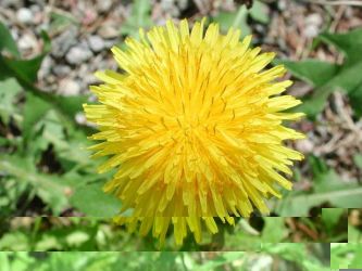
would have lower discriminative power than purely rota-             kernel for classification as a linear combination of base ker-
tionally invariant ones.                                            nels with positive weights while enforcing sparsity.
   An ideal solution would be for every descriptor to have              The body of work on learning distances [13,17,30,32,37,
a continuously tunable meta parameter controlling its level         39,41] is also relevant to our problem. In addition, boosting
of invariance. By varying the parameter, one could gener-           has been particularly successful at learning distances and
ate an infinite set of base descriptors spanning the complete       features optimised for classification and related tasks [44].
range of the trade-off and, from this set, select the single        A recent survey of the state-of-the-art in learning distances
base descriptor corresponding to the optimal trade-off level.       can be found in [19].
The optimal descriptor’s kernel matrix should have the same             There has also been a lot of work done on learning in-
structure as the ideal kernel (essentially corresponding to         variances in an unsupervised setting, see [22, 43, 49] and
zero intra-class and infinite inter-class distances) in kernel      references within. In this scenario, an object is allowed to
target alignment [15]. Unfortunately, most descriptors don’t        transform over time and a representation invariant to such
have such a continuously tunable parameter.                         transformations is learnt from the data. These methods are
   It is nevertheless possible to discretely sample the levels      not directly applicable to our problem as they are unsuper-
of invariance and generate a finite set of base descriptors.        vised and generally focus on learning invariances without
For instance, by selectively taking the maximum response            regard to discriminative power.
over scale or orientation or other transformations of a ba-             One might also try and learn an optimal descriptor di-
sic filter one can generate base descriptors that are scale in-     rectly [21, 27, 36, 48] for classification. However, our pro-
variant, rotation invariant, etc. Alternatively, one can even       posed solution has two advantages. First, by combining ker-
start with different descriptors which achieve different lev-       nels, we never need to work in combined high dimensional
els of the trade-off. The optimal descriptor can still be ap-       descriptor space with all its associated problems. By effec-
proximated, not by selecting one of the base descriptors, but       tive regularisation, we are also able to avoid the over-fitting
rather by taking their combination. However, approximat-            problem typical of such high dimensional spaces. Second,
ing the ideal kernel via kernel target alignment is no longer       we are able to combine heterogeneous sources of data, such
appropriate as the method is not geared for classification.         as shape, colour and texture.
   Our solution instead is to combine a minimal set of base             The idea of combining descriptors has been explored
descriptors specifically for classification. The theory is de-      in [8,25,33,51]. Unfortunately, these methods are not based
veloped in Section 3 but for an intuitive explanation let us        on learning. In [25, 51] a fixed combination of descriptors
return to our 4 versus 9 example. Starting with base descrip-       is tried with all descriptors being equally weighted all the
tors that are rotationally invariant, scale invariant, affine in-   time. In [8, 33] a brute force search is performed over a
variant etc., our solution is to approximate the optimal de-        validation set to determine the best descriptor weights.
scriptor by combining the rotationally invariant descriptor             Finally, the idea of a trade-off between invariance and
with just the scale invariant one. The combined descriptor          discriminative power is well known and is explored theo-
would have neither invariance in full. As a result, the dis-        retically in [40]. However, rather than learning the actual
tance between a digit and its rotated copy would no longer          trade-off, their proposed randomised invariants solution is
be zero, but would still be tolerably small. Similarly, small       to add noise to the training set features. The noise parame-
scale changes would lead to increased, small non-zero dis-          ters, corresponding to the trade-off, have to be hand tuned.
tances within class. However, the combined distance be-             In this paper, we automatically learn both the trade-off as
tween classes would also be increased and by a sufficient           well as the optimal kernel for classification.
enough margin to ensure good classification.
                                                                    3. Learning the Trade-Off
2. Related Work
                                                                        We start with Nk base descriptors and associated dis-
    Our work builds on recent advances in kernel learning.          tance functions f1 , . . . , fNk . Each descriptor achieves a dif-
It is also related to work on learning distance functions as        ferent trade-off between discriminative power and invari-
well as descriptor optimisation and combination.                    ance on the specified task. The descriptors and distance
    The goal of kernel learning is to learn a kernel which          functions are then “kernelised” to yield base kernels matri-
is optimal for the specified task. Much progress has been           ces K1 , . . . , KNk . There are many ways of converting dis-
made recently in this field and solutions have been proposed        tances to inner products and one is free to choose whichever
based on kernel target alignment [15], multiple kernel learn-       embedding is most suitable. We simply set Kk (x, y) =
ing [3, 24, 35, 42, 52], hyperkernels [34, 45], boosted ker-        exp(−γk fk (x, y)) taking care to ensure that the kernel ma-
nels [14, 20] and other methods [2, 9]. These approaches            trices are strictly positive definite.
mainly differ in the cost function that is optimised. Of par-           Given the base kernels, the P optimal descriptor’s kernel is
ticular interest are [3, 4, 35, 42] as each learns the optimal      approximated as Kopt = k dk Kk where the weights d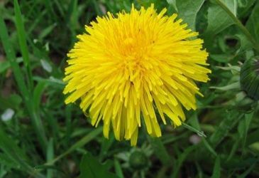
correspond to the trade-off level. The optimisation is car-      strategy of [12, 35]. In their method, the primal is reformu-
ried out in an SVM framework so as to achieve the best           lated as Mind T (d) subject to d ≥ 0 and Ad ≥ p, where
classification on the training set, subject to regularisation.                                   1 t           t      t
We set up the following primal cost function                          T (d) =        Minw,ξ      2 w w + C1 ξ + σ d             (8)
                                                                                    subject to   yi (wt φ(xi ) + b) ≥ 1 − ξi    (9)
                         1 t
        Min              2w w   + C1t ξ + σ t d            (1)                                   ξ≥0                           (10)
        w,d,ξ

   subject to          yi (wt φ(xi ) + b) ≥ 1 − ξi         (2)      The strategy is to minimise T using projected gradient
                         ξ ≥ 0, d ≥ 0, Ad ≥ p              (3)   descent via the iteration dn+1 = dn − ǫn ∇T taking care
                                  P                              to ensure that the constraints dn+1 ≥ 0 and Adn+1 ≥ p
       where      φ (xi )φ(xj ) = k dk φtk (xi )φk (xj )
                   t
                                                           (4)
                                                                 are satisfied. The important step then is calculating ∇T . In
    The objective function (1) is near identical to the stan-    order to do so, we look to the dual of T which is
dard l1 C-SVM objective. Given the misclassification                                                  P
                                                                   W (d) = Max 1t α + σ t d − 12 k dk αt YKk Yα (11)
penalty C, it maximises the margin while minimising the                         α

hinge loss on the training set {(xi , yi )}. The only addition          subject to            0 ≤ α ≤ C, 1t Yα = 0             (12)
is an l1 regularisation on the weights d since we would like
                                                                     By the principle of strong duality T (d) = W (d). Fur-
to discover a minimal set of invariances. Thus, most of the
                                                                 thermore, if α∗ maximises W , then [7] have shown that W
weights will be set to zero depending on the parameters σ
                                                                 is differentiable if α∗ is unique (which it is in our case since
which encode our prior preferences for descriptors. The l1
                                                                 all the kernel matrices are strictly positive definite). Finally,
regularisation thus prevents overfitting if many base kernels
                                                                 as proved in Lemma 2 of [12], W can be differentiated with
are included since only a few will end up being used. Also,
                                                                 respect to d as if α∗ did not depend on d. We therefore get
it can be shown that the quantity 21 wt w is minimised by
increasing the weights and letting the support vectors tend                 ∂T    ∂W
to zero. The regularisation prevents this from happening                        =     = σk − 21 α∗t YKk Yα∗                    (13)
                                                                            ∂dk   ∂dk
and can therefore be seen as not letting the weights become
too large. This could also be achieved by requiring that the         The minimax algorithmP   proceeds in two stages. In the
weights sum to unity but we prefer not to do this as it re-      first, d and therefore K = dk Kk are fixed. Since σ t d is
stricts the search space.                                        a constant, W is the standard SVM dual with kernel matrix
    The constraints are also similar to the standard SVM         K. Any large scale SVM solver of choice can therefore be
formulation. Two additional constraints have been incor-         used to maximise W and obtain α∗ . In the second stage,
porated. The first, d ≥ 0, ensures that the weights are          T is minimised by projected gradient descent according to
interpretable and also leads to a much more efficient op-        (13). The two stages are repeated until convergence [11] or
timisation problem. The second, Ad ≥ p, with some                a maximum number of iterations is reached at which point
restrictions, lets us encode our prior knowledge about the       the weights d and support vectors α∗ have been solved for.
problem.PThe final condition (4) is just a restatement of            A novelPpoint x can now be classified as ±1 by determin-
Kopt = k dk Kk using the non-linear embedding φ.                 ing sign( i αi yi Kopt (x, xi ) + b). To handle multi-class
                                                                 problems, both 1-vs-1 and 1-vs-All formulations are tried.
    It is straightforward to derive the corresponding dual
                                                                 For 1-vs-1, the task is divided into pairwise binary classifi-
problem which turns out to be:
                                                                 cation problems and a novel point is classified by taking the
                                                                 majority vote over classifiers. For 1-vs-All, one classifier is
           Max                 1t α + pt δ                 (5)
            α,δ                                                  learnt per class and a novel point is classified according to
      subject to 0 ≤ δ, 0 ≤ α ≤ C, 1t Yα = 0               (6)   its maximal distance from the separating hyperplanes.
                       1 t                     t
                       2 α YKk Yα    ≤ σk − δ Ak           (7)
                                                                 4. Experimentation
where the non-zero αs correspond to the support vectors,             In this section, we apply our method to the UIUC tex-
Y is a diagonal matrix with the labels on the diagonal and       tures [25], Oxford flowers [33] and Caltech 101 object cat-
Ak is the k th column of A.                                      egorisation [16] databases. Since we would like to test how
   The dual is convex with a unique global optimum. It is an     general the technique is, we assume that no prior knowledge
instance of a Second Order Cone Program [10] and can be          is available and that no descriptor is a priori preferable to
solved relatively efficiently by off-the-shelf numerical opti-   any other. We therefore set σk to be constant for all k and do
misation packages such as SeDuMi [1].                            not make use of the constraints Ad ≥ p (unless otherwise
   However, in order to tackle large scale problems involv-      stated). The only parameters left to be set are C, the mis-
ing hundreds of kernels we adopt the minimax optimisation        classification penalty, and the kernel parameters γk . These
parameters are not tweaked. Instead, C is set to 1000 for all      Invariance                         1NN            SVM (1-vs-1)
classifiers and databases and γk is set as in [51].                None (Patch)                  82.39 ± 1.58%       91.46 ± 1.13%
   To present comparative results, we tried the Multiple           None (MR)                     82.18 ± 1.51%       91.16 ± 1.05%
Kernel Learning SDP formulation of [24]. However, as [24]          Rotation (Patch)              97.83 ± 0.63%       98.18 ± 0.43%
does not enforce sparsity and the results were 5% worse on         Rotation (MR)                 93.00 ± 1.04%       96.69 ± 0.74%
the Caltech database we didn’t explore the method further.         Rotation (Fractal)            94.96 ± 0.91%       97.24 ± 0.76%
Instead, we compare our method to the Multiple Kernel              Scale (MR)                    76.77 ± 1.77%       87.04 ± 1.57%
Learning Block l1 regularisation method of [4] for which           Similarity (MR)               90.35 ± 1.15%       95.12 ± 0.95%
code is publicly available. All experimental results are cal-      Bi-Lipschitz (Fractal)        95.40 ± 0.92%       97.19 ± 0.52%
culated over 20 random train/test splits of the data except       Table 1. Classification results on the UIUC texture dataset. The
for 1-vs-All results which are calculated over 3 splits.          MKL-Block l1 method of [4] achieves 96.94 ± 0.91% for 1-vs-1
                                                                  classification when combining all the descriptors. Our results are
                                                                  98.76 ± 0.64% (1-vs-1) and 98.9 ± 0.68% (1-vs-All).
4.1. UIUC textures
    The UIUC texture database [25] has 25 classes and 40
images per class. The database contains materials imaged             For classification, the testing methodology is kept the
under significant viewpoint variations and also contains fab-     same as in [51] – 20 images per class are used for training
rics which display folds and have non-rigid surface defor-        and the other 20 for testing. Table 1 lists the classification
mations. A priori, it is hard to tell what is the right level     results. Our results are comparable to the 98.70 ± 0.4%
of invariance for this database. Affine invariance is proba-      achieved by the state-of-the-art [51]. What is interesting
bly helpful given the significant viewpoint changes. Higher       is that our performance has not decreased below that of
levels of invariance might also be needed to characterise         any single descriptor despite the inclusion of specialised de-
fabrics and handle non-affine deformations. However, [51]         scriptors having scale and no invariance. These descriptors
concluded that similarity invariance is better than either        have poor performance in general. However, our method
scale or affine invariance for this database. Then again,         automatically sets their weights to zero most of the time
our results indicate that even better performance can be ob-      and uses them only when they are beneficial for classifica-
tained by sticking to rotationally invariant descriptors. This    tion. Had the equally weighted combination scheme of [51]
reinforces the observation that it is not always straight for-    been used, these descriptors would have been brought into
ward to pinpoint the required level of invariance.                play all the time and the resulting accuracy drops down
                                                                  to 96.79 ± 0.86%. In each of the 20 train/test splits,
    For this database, we start with a standard patch descrip-
tor having no invariance but then take different transforms
to derive 7 other base descriptors achieving different lev-
els of the trade-off. The first descriptor is obtained by lin-
early projecting the patch onto the MR filters [47] (see Fig-
ure 1). Subsequent rotation, scale and similarity invariant
descriptors are obtained by taking the maximum response
of a basic filter over orientation, scale or both. This is sim-
ilar to [38] where the maximum response is taken over po-
sition to achieve translation invariance. MR filter responses
can also be used to derive fractal based bi-Lipschitz (includ-       Class 23          Class 3           Class 7          Class 4
ing affine, perspective and non-rigid surface deformations)       Figure 2. 1-vs-1 weights learnt on the UIUC database: Both
invariant and rotation invariant descriptors [46]. Finally,       class 23 and class 3 exhibit significant variation. As a result, bi-
patches can directly yield rotation invariant descriptors by      Lipschitz invariance gets a very high weight when distinguishing
                                                                  between these two classes while all the other weights are 0. How-
aligning them according to their dominant orientation.
                                                                  ever class 7 is simpler and the main source of variability is rota-
                                                                  tion. Thus, full bi-Lipschitz invariance is no longer needed when
                                                                  distinguishing between class 23 and class 7. It can therefore be
                                                                  traded-off with a more discriminative descriptor. This is reflected
                                                                  in the learnt weights where rotation invariance gets a high weight
                                                                  of 1.46 while bi-Lipschitz invariance gets a small weight of 0.22.
                                                                  Bi-Lipschitz invariance isn’t set to 0 as class 23 would start get-
                                                                  ting misclassified. However, if class 23 were replaced with the
                                                                  simpler class 4, which primarily has rotations, then bi-Lipschitz
                                                                  invariance is no longer necessary. Thus, when distinguishing class
            Figure 1. The extended MR8 filter bank.               7 from class 4, rotation invariance is the only feature used.
Descriptor 1NN SVM (1-vs-1)
Shape 53.30 ± 2.69% 68.88 ± 2.04%
Colour 47.32 ± 2.59% 59.71 ± 1.95%
Texture 39.36 ± 2.43% 59.00 ± 2.14%
Table 2. Classification results on the Oxford flowers dataset. The
MKL-Block l1 method of [4] achieves 77.84 ± 2.13% for 1-vs-1
classification when combining all the descriptors. Our results are
80.49 ± 1.97% (1-vs-1) and 82.55 ± 0.34% (1-vs-All).
Class 10 vs 25 Class 8 vs 15
Similarity Similarity
Normalised Weight
Normalised Weight
Bi−Lipschitz Bi−Lipschitz start with shape, colour and texture distances between every
1 1
image pair, provided directly by the authors of [33]. Test-
ing is also carried out according to the methodology of [33].
0.5 0.5
Thus, for each class, 40 images are used for training, 20 for
0 0
validation and 20 for testing. We make no use of the valida-
0 20 40 60 80 0 20 40 60 80 tion set as all our parameters have already been set. Table 2
Training set size Training set size
(a) (b) lists the classification results. Our results are better than the
Figure 3. Column (a) shows images from classes 10 and 25 and individual base kernels and are also better than the MKL-
the variation in learnt weights as the training set size is increased Block l1 formulation on each of the 20 train/test splits.
for this pairwise classification task. A similar plot for classes 8 Figure 4 (a) plots the distribution of the learnt shape and
and 15 is shown in (b). When the training set size is small, a colour weights for all 136 pairwise classifiers in the 1-vs-
higher level of invariance (bi-Lipschitz) is needed. As the training 1 formulation. Normalised texture weights are shown as
set size grows, a less invariant and more discriminative descriptor colour codes to emphasise that they are relatively small.
(similarity) is preferred and automatically learnt by our method.
Note that the weights don’t favour either just shape or just
The trends, though not identical, are similar in both (a) and (b)
indicating that the tasks could be related. Inspecting the two class
colour features. An entire set of weights is learnt, span-
pairs indicates that while they are visually distinct, they do share ning the full range from shape to colour. While a person
the same types of variations (apart from the fabric crumpling). could correctly predict which is the more important feature
by looking at the images, they would be hard pressed to
achieve the precise trade-off.
learning the descriptors using our method outperformed The relative importance of the learnt 1-vs-1 weights
equally weighted combinations (as well as the MKL-Block is curious. Shape turns out to be the dominant feature
l1 method). Figure 2 shows how the learnt weights cor- in 38.24% of the pairwise classification tasks, colour in
respond visually to the trade-offs between different classes 60.29% and texture in 1.47%. This is surprising, since ac-
while Figure 3 shows that the learnt weights change sensi- cording to the individual SVM classification results in Ta-
bly as the training set size is varied. ble 2, shape is the best single feature and texture is nearly as
good as colour. Texture features are probably ignored in our
4.2. Oxford Flowers formulation as they are very strongly correlated with shape
The Oxford flowers database [33] contains 17 different features (both are edge based). The l1 regularisation prefers
categories of flowers and each class has 80 images. Classi- minimal feature sets with small weights and so gives tex-
fication is carried out on the basis of vocabularies of visual ture either zero or low weights. Forcing the texture weights
words of shape, colour and texture descriptors in [33]. The to be high (by constraining them to be higher than colour
background in each image is removed using graph cuts so using the constraint term Ad ≥ p) improves the overall
as to extract features from the flowers alone and not from
the surrounding vegetation. Shape distances between two
images are calculated as the χ2 statistic between the nor- 6
0.5 6 6
Bluebells
Sunflowers
malised frequency histograms of densely sampled, vector 4 0.4
4
Daisies
4
Crocuses
Colour
Colour
0.3
quantised SIFT descriptors [29] of the two images. Sim-
Colour
2 2
0.2 2
ilarly, colour distances are computed over vocabularies of 0 0.1
0 0
HSV descriptors and texture over MR8 filter responses [47]. 0 2 4 6
0
0 2 4 6 0 2 4 6
Shape Shape Shape
Cue combination fits well within our framework as one (a) (b) (c)
can think of an ideal colour descriptor as being very highly Figure 4. The distribution of the learnt shape and colour weights
discriminating on the basis of an object’s colour but invari- on the Oxford flowers dataset: (a) 1-vs-1 pairwise weights for all
ant to changes in the object’s shape or texture. Similar argu- the classes; (b) 1-vs-1 weights for Sunflowers and Daisies; and (c)
ments hold for shape and texture descriptors. We therefore Bluebells and Crocuses.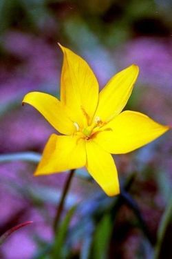
classification tasks (see Figure 6). Such knowledge could
be useful for learning and transferring priors.
Finally, since only three descriptors are used on this data-
base, an exhaustive search can be performed on a validation
set for the best combination of weights. However, it was no-
ticed that performing a brute force search over every class
Dandelions Wild Tulips Crocuses Cowslips Irises
pair lead to overfitting. If ties were not resolved properly,
the overall classification performance could be as poor as
Figure 5. 1-vs-1 weights learnt on the Oxford dataset: Dande-
lions and Wild Tulips are both yellow and therefore colour is a
60%. We therfore enforced that, in the 1-vs-1 formulation,
nuisance parameter to which we should be invariant. However, all pairwise classifiers should have the same weights and
shape is a good discriminator for these flowers. This is reflected performed a brute force search again. The best weights re-
in the weights which are learnt to be shape=3.94, colour=0 and sulted in an accuracy of 80.62 ± 1.65% which is similar to
texture=0. When the task changes to distinguishing Dandelions our results. A 1-vs-All brute force search couldn’t be per-
from Crocuses, shape becomes a poor discriminator (Crocuses formed as it was computationally too expensive.
have large variability) but colour becomes good. However, Cro-
cuses also have some yellow which causes confusion. To compen- 4.3. Caltech 101 Object Categorisation
sate for this, shape invariance is traded-off for increased discrimi-
nation and the learnt weights are shape=0.42, colour=2.46 and tex- The Caltech 101 database [16] contains images of 101
ture=0. When distinguishing Cowslips from Irises, all three fea- categories of objects as well as a background class. The
tures are used and the weights are shape=1.48, colour=2.00 and database is very challenging as it contains classes with sig-
texture=1.36. As can be seen, colour is good at characterising nificant shape and appearance variations (Ant, Chair) as
Cowslips (which are always yellow) but not sufficient for distin-
well as classes with roughly fixed shape but considerably
guishing them from Irises which might also be yellow. Shape and
texture features are also not sufficient by themselves due to the
varying appearance (Butterfly, Watch) or vice-versa (Leop-
large intra-class variability. However, combining all three features ard, Panda). We therefore combine 6 shape and appearance
in the right proportion leads to good discrimination. features for this dataset.
The first two shape descriptors correspond to equations
(1) and (2) in [50] and are based on Geometric Blur [5].
1-vs-1 accuracy marginally to 81.12 ± 2.09%. Pairwise image distances for these were provided directly
A few classes along with their learnt pairwise weights are by the authors for the training and test images used in their
shown in Figure 5. Keeping one class fixed and varying the paper. For the first descriptor, GB, the distance between
other results in the weights changing according to changes two images is fGB (I1 , I2 ) = DA (IP A
1 → I2 ) + D (I2 →
in perceptual cues. Since the learnt weights provide a layer m
I1 ) where DA (I1 → I2 ) = (1/m) i=1 minj=1..n kFi1 −
of abstraction, one can use them to reason about the given Fj2 k. Fi1 and Fj2 are Geometric Blur features in the two
classification problem. For instance, Figure 4 (b) and (c) images. The texture term in (1) in [50] is not used. The
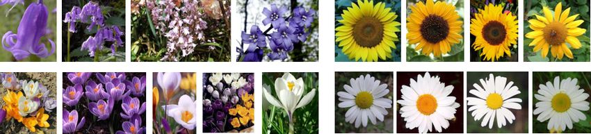
plot the distribution of all 1-vs-1 weights for Bluebells and second descriptor, GBDist, corresponding to (2) in [50]. It
Crocuses and Sunflowers and Daisies respectively. The dis- is very similar to GB except that DA now incorporates an
tributions of Bluebells and Crocuses are similar as are that additional first-order geometric distortion term.
of Sunflowers and Daisies but the two sets are distinct from We also incorporate the four descriptors used in [8].
each other. This shows that these categories form related The two appearance features, AppGray and AppColour, are
based on SIFT descriptors sampled on a regular grid. At
each point on the grid, SIFT descriptors are computed us-
Descriptor 1NN SVM (1-vs-1)
GB 39.67 ± 1.02% 57.33 ± 0.94%
Bluebells (top) & Crocuses Sunflowers (top) & Daisies GBDist 45.23 ± 0.96% 59.30 ± 1.00%
Figure 6. Learning related tasks: Bluebells and Crocuses share AppGray 42.08 ± 0.81% 52.83 ± 1.00%
similar sets of invariances. Apart from some cases, they require AppColour 32.79 ± 0.92% 40.84 ± 0.78%
higher degrees of shape invariance and can be distinguished well Shape180 32.01 ± 0.89% 48.83 ± 0.78%
on the basis of their colour. Sunflowers and Daisies are neither Shape360 31.17 ± 0.98% 50.63 ± 0.88%
distinctive in shape nor in colour from all the other classes. They Table 3. Classification results on the Caltech 101 dataset. The
form another related pair in that sense. Since the flowers in each MKL-Block l1 method of [4] achieves 76.55 ± 0.84% for 1-vs-
related pair are visually different, it might be hard to establish such 1 classification when combining all the descriptors. Our results
relationships by visual inspection alone. are 78.43 ± 1.05% (1-vs-1) and 87.82 ± 1.00% (1-vs-All).
Starting with base descriptors which achieve different levels
                                                                          of the trade-off, our solution is to combine them optimally
                                                                          in a kernel learning framework. The learnt kernel yields
                     (a)                                   (b)            superior classification results while the learnt weights cor-
Figure 7. In (a) the three classes, Pizza, Soccer ball and Watch, all     respond to the trade-off and can be used for meta level tasks
consist of round objects and so the learnt weights do not use shape       such as transfer learning or reasoning about the problem.
for any of these class pairs. In (b) both Butterfly and Electric guitar      Our framework has certain attractive properties. It ap-
have significant within class appearance variation. However, their        pears to be general and capable of handling diverse classi-
shape remains much the same within class and is distinct between          fication problems. No hand tuning of parameters was re-
the classes. As such, only shape is used to distinguish these two
                                                                          quired. In addition, it can be used to combine heteroge-
classes from each other.
                                                                          neous sources of data. This is particularly relevant in cases
                                                                          where human intuition about the right levels of invariance
ing 4 fixed scales. These are then vector quantised to form a             might fail – such as when combining audio, video and text.
vocabulary of visual words. Images are represented as a bag               Another advantage is that the method can work with poor,
of words and similarity between two images is given by the                or highly specialised, descriptors. This is again useful in
spatial pyramid kernel [26]. While AppGray is computed                    cases when the right levels of invariance are not known a
from gray scale images, AppColour is computed from an                     priori and we would like to start with many base descrip-
HSV representation. The two shape features, Shape180 and                  tors. Also, it appears that we get similar (Oxford Flowers)
Shape360, are represented as histograms of oriented gradi-                or better (Caltech 101) results as compared to brute force
ents and matched using the spatial pyramid kernel. Gradi-                 search over a validation set. This is particularly encour-
ents are computed using the Canny edge detector followed                  aging since a brute force search can be computationally ex-
by Sobel filtering. They are then discretized into the orienta-           pensive. In addition, in the very small training set size limit,
tion histogram bins with soft voting. The primary difference              it might not be feasible to hold out training data to form a
between the two descriptors is that Shape180 is discretized               validation set and one also risks overfitting. Finally, our per-
into bins in the range [0, 180] and Shape360 into [0, 360].               formance was generally better than that of the MKL-Block
Details can be found in [8]. Note that since the gradients                l1 method while also enjoying the advantage of scaling up
are computed at both boundary and texture edges these de-                 to large problems as long as efficient solvers for the corre-
scriptors represent both local shape and local texture.                   sponding single kernel problem are available.
    To evaluate classification performance, we stick to the
methodology adopted in [6, 50]. Thus, 15 images are ran-                  Acknowledgements
domly selected from all 102 class (i.e. including the back-
ground) for training and another random 15 for testing.                      We are very grateful to the following for providing ker-
Classification results using each of the base descriptors as              nel matrices and for many helpful discussions: P. Anandan,
well as their combination are given in Table 3 and Figure 7               Anna Bosch, Rahul Garg, Varun Gulshan, Jitendra Malik,
gives a qualitative feel of the learnt weights.                           Maria-Elena Nilsback, Patrice Simard, Kentaro Toyama,
    To compare our results to the state-of-the-art, note                  Hao Zhang and Andrew Zisserman.
that [50] combine shape and texture features to obtain
59.08 ± 0.37% and [18] combine colour features in addi-                   References
tion to get 60.3 ± 0.70%. Kernel target alignment is used
                                                                           [1] http://sedumi.mcmaster.ca/.
by [28] to combine 8 kernels based on shape, colour tex-
                                                                           [2] A. Argyriou, C. A. Micchelli, and M. Pontil. Learning con-
ture and other cues. Their results are 59.80%. In [23], a                      vex combinations of continuously parameterized basic ker-
performance of 57.83% is achieved by combining 12 ker-                         nels. In COLT, 2005.
nels using the MKL-Block l1 method. In [8], a brute force                  [3] F. R. Bach, G. R. G. Lanckriet, and M. I. Jordan. Multiple
search is performed over a validation set to learn the best                    kernel learning, conic duality, and the SMO algorithm. In
combination of their 4 kernels in a 1-vs-All formulation.                      NIPS, 2004.
When training and testing on 15 images for 101 categories                  [4] F. R. Bach, R. Thibaux, and M. I. Jordan. Computing regu-
(i.e. excluding background) they record an overall classifi-                   larization paths for learning multiple kernels. In NIPS, 2004.
cation accuracy of 71.4 ± 0.8%. Using the same 4 kernels                   [5] A. Berg and J. Malik. Geometric blur for template matching.
but testing on all 102 categories we obtain 79.85 ± 0.04%.                     In CVPR, volume 1, pages 607–614, 2001.
                                                                           [6] A. C. Berg, T. L. Berg, and J. Malik. Shape matching and
5. Conclusions                                                                 object recognition using low distortion correspondence. In
                                                                               CVPR, volume 1, pages 26–33, San Diego, California, 2005.
   In this paper, we developed an approach for learning the                [7] J. F. Bonnans and A. Shapiro. Perturbation Analysis of Op-
discriminative power-invariance trade-off for classification.                  timization Problems. 2000.
[8] A. Bosch, A. Zisserman, and X. Munoz. Representing shape          [32] E. Miller, N. Matsakis, and P. Viola. Learning from one
     with a spatial pyramid kernel. In Proc. CIVR, 2007.                    example through shared densities on transforms. In CVPR,
 [9] O. Bousquet and D. J. L. Herrmann. On the complexity of                pages 464–471, 2000.
     learning the kernel matrix. In NIPS, pages 399–406, 2002.         [33] M.-E. Nilsback and A. Zisserman. A visual vocabulary for
[10] S. Boyd and L. Vandenberghe. Convex Optimization. 2004.                flower classification. In CVPR, volume 2, pages 1447–1454,
[11] P. Calamai and J. More. Projected gradient methods for lin-            New York, New York, 2006.
     early constrained problems. Mathematical Programming,             [34] C. S. Ong, A. J. Smola, and R. C. Williamson. Learning the
     39(1):93–116, 1987.                                                    kernel with hyperkernels. JMLR, 6:1043–1071, 2005.
[12] O. Chapelle, V. Vapnik, O. Bousquet, and S. Mukherjee.            [35] A. Rakotomamonjy, F. Bach, S. Canu, and Y. Grandvalet.
     Choosing multiple parameters for Support Vector Machines.              More efficiency in multiple kernel learning. In ICML, 2007.
     Machine Learning, 46:131–159, 2002.                               [36] T. Randen and J. H. Husoy. Optimal filter-bank design for
[13] S. Chopra, R. Hadsell, and Y. LeCun. Learning a similarity             multiple texture discrimination. In ICIP, volume 2, pages
     metric discriminatively, with application to face verification.        215–218, Santa Barbara, California, 1997.
     In CVPR, volume 1, pages 26–33, 2005.                             [37] L. Ren, G. Shakhnarovich, J. K. Hodgins, P. Hanspeter, and
[14] K. Crammer, J. Keshet, and Y. Singer. Kernel design using              P. Viola. Learning silhouette features for control of human
     boosting. In NIPS, pages 537–544, 2002.                                motion. ACM Trans. Graph, 24(4):1303–1331, 2005.
[15] N. Cristianini, J. Shawe-Taylor, A. Elisseeff, and J. Kandola.    [38] T. Serre, L. Wolf, S. Bileschi, M. Riesenhuber, and T. Pog-
     On kernel-target alignment. In NIPS, 2001.                             gio. Robust object recognition with cortex-like mechanisms.
[16] L. Fei-Fei, R. Fergus, and P. Perona. One-shot learning of             IEEE PAMI, 2007. To appear.
     object categories. IEEE PAMI, 28(4):594–611, 2006.                [39] G. Shakhnarovich, P. Viola, and T. J. Darrell. Fast pose es-
[17] A. W. Fitzgibbon and A. Zisserman. On affine invariant clus-           timation with parameter-sensitive hashing. In ICCV, pages
     tering and automatic cast listing in movies. In Proc. ECCV,            750–757, 2003.
     volume 3, pages 304–320, Copenhagen, Denmark, 2002.               [40] X. Shi and R. Manduchi. Invariant operators, small samples,
[18] A. Frome, Y. Singer, and J. Malik. Image retrieval and recog-          and the bias-variance dilemma. In CVPR, volume 2, pages
     nition using local distance functions. In NIPS, 2006.                  528–534, 2004.
[19] T. Hertz. Learning Distance Functions: Algorithms and Ap-         [41] P. Simard, Y. LeCun, J. Denker, and B. Victorri. Transfor-
     plications. PhD thesis, 2006.                                          mation invariance in pattern recognition – tangent distance
[20] T. Hertz, A. Bar-Hillel, and D. Weinshall. Learning a kernel           and tangent propagation. International Journal of Imaging
     function for classification with small training samples. In            System and Technology, 11(2):181–194, 2001.
     ICML, pages 401–408, Pittsburgh, USA, 2006.                       [42] S. Sonnenburg, G. Raetsch, C. Schaefer, and B. Schoelkopf.
[21] A. K. Jain and K. Karu. Learning texture discrimination                Large scale multiple kernel learning. JMLR, 7:1531–1565,
     masks. IEEE PAMI, 18(2):195–205, 1996.                                 2006.
[22] A. Kannan, N. Jojic, and B. J. Frey. Fast transformation-         [43] M. W. Spratling. Learning viewpoint invariant percep-
     invariant component analysis. IJCV, Submitted.                         tual representations from cluttered images. IEEE PAMI,
                                                                            27(5):753–761, 2005.
[23] A. Kumar and C. Sminchisescu. Support kernel machines
                                                                       [44] K. Tieu and P. Viola. Boosting image retrieval. IJCV, 56(1-
     for object recognition. In ICCV, 2007.
                                                                            2):17–36, 2004.
[24] G. R. G. Lanckriet, N. Cristianini, P. Bartlett, L. El Ghaoui,
                                                                       [45] I. W. Tsang and J. T. Kwok. Efficient hyperkernel learning
     and M. I. Jordan. Learning the kernel matrix with semidefi-
                                                                            using second-order cone programming. IEEE Trans. Neural
     nite programming. JMLR, 5:27–72, 2004.
                                                                            Networks, 17(1):48–58, 2006.
[25] S. Lazebnik, C. Schmid, and J. Ponce. A sparse tex-
                                                                       [46] M. Varma and R. Garg. Locally invariant fractal features for
     ture representation using local affine regions. IEEE PAMI,
                                                                            statistical texture classification. In ICCV, 2007.
     27(8):1265–1278, 2005.
                                                                       [47] M. Varma and A. Zisserman. A statistical approach to texture
[26] S. Lazebnik, C. Schmid, and J. Ponce. Beyond bags of
                                                                            classification from single images. IJCV, 2005.
     features: Spatial pyramid matching for recognizing natural
                                                                       [48] S. Winder and M. Brown. Learning local image descriptors.
     scene categories. In CVPR, volume 2, pages 2169–2178,
                                                                            In CVPR, 2007.
     New York, New York, 2006.
                                                                       [49] T. Wiskott, L. Sejnowski. Slow feature analysis: Un-
[27] Y. LeCun, L. Bottou, Y. Bengio, and P. Haffner. Gradient-
                                                                            supervised learning of invariances. Neural Computation,
     based learning applied to document recognition. Proceed-
                                                                            14(4):715–770, 2002.
     ings of the IEEE, 86(11):2278–2324, 1998.
                                                                       [50] H. Zhang, A. Berg, , M. Maire, and J. Malik. SVM-KNN:
[28] Y. Y. Lin, T. Y. Liu, and C. S. Fuh. Local ensemble kernel
                                                                            Discriminative nearest neighbor classication for visual cate-
     learning for object category recognition. In CVPR, 2007.
                                                                            gory recognition. In CVPR, pages 2126–2136, 2006.
[29] D. G. Lowe. Distinctive image features from scale-invariant
                                                                       [51] J. Zhang, M. Marszalek, S. Lazebnik, and C. Schmid. Local
     keypoints. IJCV, 60(2):91–110, 2004.
                                                                            features and kernels for classification of texture and object
[30] S. Mahamud and M. Hebert. The optimal distance measure
                                                                            categories: A comprehensive study. IJCV, 2007.
     for object detection. In CVPR, pages 248–255, 2003.
                                                                       [52] A. Zien and C. S. Ong. Multiclass multiple kernel learning.
[31] K. Mikolajczyk and C. Schmid. A performance evaluation
                                                                            In ICML, pages 1191–1198, 2007.
     of local descriptors. IEEE PAMI, 27(10):1615–1630, 2005.
You can also read