Data-driven design of deployable structures: Literature review and multi-criteria optimization approach** - De Gruyter
←
→
Page content transcription
If your browser does not render page correctly, please read the page content below
Curved and Layer. Struct. 2021; 8:241–258

Research Article

Milan Dragoljevic*, Salvatore Viscuso, and Alessandra Zanelli

Data-driven design of deployable structures:
Literature review and multi-criteria optimization
approach**
https://doi.org/10.1515/cls-2021-0022
Received Sep 15, 2020; accepted Jan 28, 2021
                                                                        1 Introduction
Abstract: Classification and development of the deploy-                 1.1 Deployable structures
able structures is an ongoing process that started at the
end of 20th century and is getting more and more attention              Among the architectural structures, there are special ones
throughout 21st . With the development of the technology,               that have the ability to change their shape, position in space
constructive systems and materials, these categorizations               and to adapt to external conditions. These are called adap-
changed – adding new typologies and excluding certain                   tive and morphing structures. A special case of these struc-
ones. This work is giving a critical review of the work done            tures which have a single degree of freedom and only two
previously and on the change of the categories. The special             possible configurations (compact and deployed) are called
interest is given to the pantographs (or scissor structures)            deployable structures. The compact and deployed config-
and the Zeigler’s dome as the form of their application. It             urations are defined a priori and thus the structure is not
is noticeable that after its introduction in 1977, the dome             conceived to respond or adapt to real-time changing sce-
was a part of the initial classification, but with the time it          narios, nor is designed to be used with different conditions
lost its place. The reason for this is the introduction of more         in a same context [1]. This is performed as a response to
efficient scissor dome structures. However, perhaps with                a variable number of requirements: emergencies, special
the use of data-driven design, this dome can be optimized               functions or changes of the environments. The other names
and become relevant again.                                              of these structures are erectable, expandable, extendible,
The second part of the paper is dedicated to the develop-               developable or unfurlable structures [2].
ment of the structural optimization algorithm for panto-                     The use of deployable structures is a part of human
graph structures and its application on the example of Zei-             society for a long time. Shelters that are easy to be trans-
gler’s dome. Besides the direct analysis, the final part in-            ported and assembled were part of the exploration or the
cludes the generative optimization algorithm which could                big movement of the tribes. Also, the military during the
help to a decision-maker in the early stages of the design              campaigns required sheltering on different terrains. Appli-
to understand and select the options for the structure.                 cations range from the Mongolian yurts to the velum of the
Keywords: deployable structures, classification, pan-                   Roman Coliseum, from Da Vinci’s umbrella to the folding
tographs, Zeigler’s dome, scissor mechanism, deployable                 chair [3]. They were used whenever there was a need for a
dome, structural optimization, generative algorithm                     temporary enclosure. However, the academic interest in the
                                                                        topic began in the second half of the 20th century. Zuk and
                                                                        Clark published in 1970 their book Kinetic Architecture that
                                                                        was the first important focus on the topic [4]. Part of their
                                                                        references is coming from the 1960s: for example Rowan J.
                                                                        Progressive architecture – p. 93 [5].
*Corresponding Author: Milan Dragoljevic: Politecnico di Mi-
lano, Dept. of Architecture, Built Environment and Construction
                                                                             Similar to the historical application, the structures to-
Engineering Via Ponzio 31, 20133 Milan, Italy;                          day are also utilized for temporary needs. These include
Email: milan.dragoljevic@polimi.it                                      emergency situations sheltering, events organization or as
Salvatore Viscuso, Alessandra Zanelli: Politecnico di Milano,           a response to the change of the environment. All the men-
Dept. of Architecture, Built Environment and Construction Engineer-     tioned situations require objects which will have a shorter
ing Via Ponzio 31, 20133 Milan, Italy
                                                                        use period compared to the conventional edifices. Because
** Paper included in the Special Issue entitled: Shell and Spatial
Structures: Between New Developments and Historical Aspects             of this, construction time should also be shortened. Consid-

  Open Access. © 2021 M. Dragoljevic et al., published by De Gruyter.            This work is licensed under the Creative Commons Attribution
4.0 License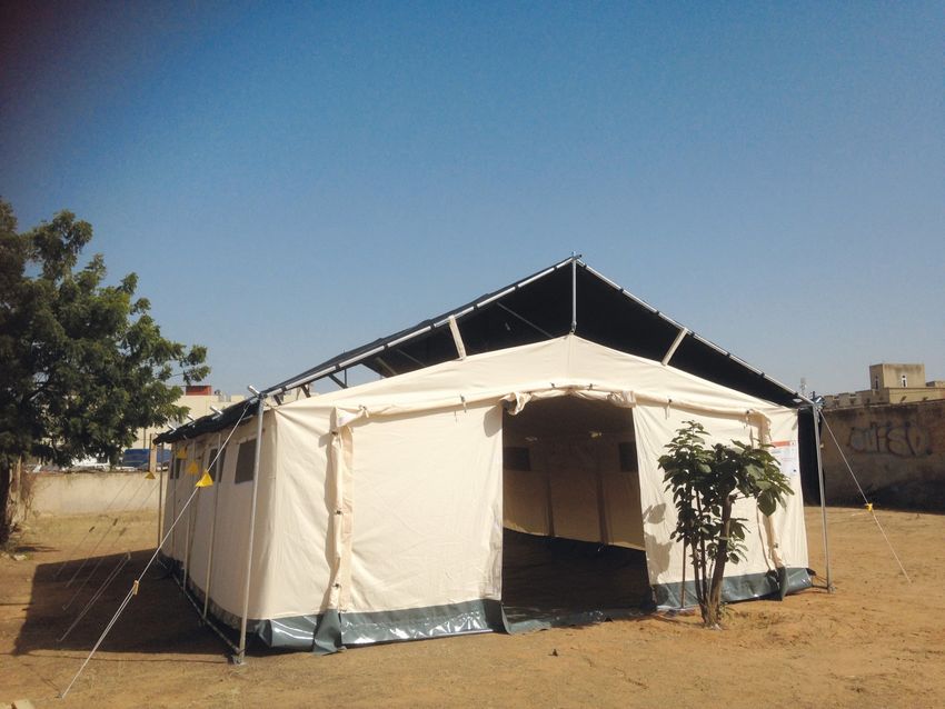
242 | M. Dragoljevic et al.
ering the emergencies, the utilization time and conditions cations presented on the chronology below (Figure 3) are
are unpredictable, so the adaptability and possibility to compared with the general classifications and therefore
re-deploy in a short time if needed plays a key role. The observed in the same period. The first partial classification
events can be organized as repetitive or on different loca- after the 1980s is a historical survey of cable and membrane
tions, that is why the time for deployment and transport is roofs by Forster [7], published in 1994 and then deepened
very important. two years later in 1996 by Mollaert [8] with the classification
of the membrane roofs. In 2001, Friedman publishes the
doctoral thesis containing the review of deployable struc-
tures [9]. Yet, this review is focused on architectural and
civil engineering applications and she specifies that it is
not a comprehensive work. She publishes a similar review
in 2011. Doroftei and Doroftei published in 2014 another
short review of deployable structures [10]. Their classifi-
cation contains 4 categories: spatial bar structures, fold-
able plate structures, strut-cable systems and membrane
systems. However, in their work, they focus mostly on the
first two classes. Puig et al. review deployable booms and
masts [11]. This work classifies them as: inflatable, tele-
scopic, coilable, shape-memory composite booms and de-
ployable truss structures. Environmental performance as
the criteria for classification is adopted by Ramzy and Fayed
in 2011 [12]. They divide deployable structures into the fol-
Figure 1: POLIMI and IFRC, T2 Multipurpose collective shelter
lowing classes: skin-unit systems, retractable elements, re-
volving buildings and biomechanical systems. Santiago-
Prowald and Baier focus on space antennas in their work
from 2013 [13]. They distinguish different approaches in the
deployment of them.
One of the first comprehensive classifications was done
by Carlos H. H. Merchan in his Master thesis published 1987
for the Massachusetts Institute of Technology (MIT) [14].
The first level division in this case is between strut and
surface elements. Linear elements as struts can resist dif-
ferent types of load (tension, compression or bending). On
the other hand, surface structures are continuous and cer-
tain of them resist only tension forces. Sliding mechanisms
(umbrella type) are mentioned in this classification, but
not in further work of other authors. As part of the surface
elements, there are inflatable or pneumatic structures, al-
though without the explanation are they air-inflated or air-
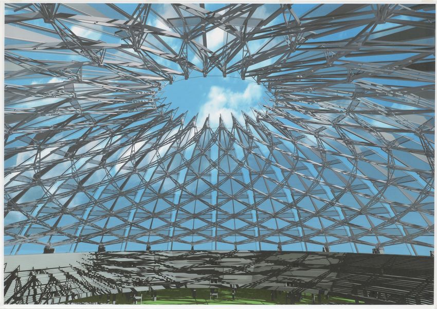
Figure 2: Chuck Hoberman, Iris Dome Project, Interior perspec- supported. Despite the extensive work on covering different
tive;1994
typologies of the deployable structures, some of them were
not mentioned, although they were invented at the time of
Considering the work on the comprehensive classifi- the writing classification – tensegrities, air-supported struc-
cation of different types of deployable structures, the ex- tures and sliding structures used for retractable roofs. This
amples started to show up from the 1980s [6]. After that, division also contains pantographs [15] under the name of
there was a big break until the 21st century, when the topic scissor hinged mechanisms.
returned to focus and new attempts to classify general de- After this, the next steps in classification are done in
ployable structures showed up. the 21st century – starting from the year 2001. Charalambos
On the other hand, for the classification of specific Gantes created the first classification in our century [16]. His
types, the work was more continuous. The partial classifi- book Deployable Structures: Analysis and Design contains
a critical overview of the deployable structures. The first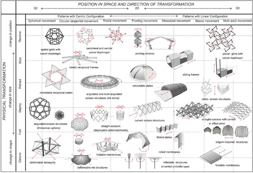
Data-driven design of deployable structures |   243

Figure 3: Chronological view of comprehensive and partial classifications of deployable structures published by now

Figure 4: Merchan’s classification of deployable structures from 1987

Figure 5: Deployable structures classification of Gantes in 2001
244 | M. Dragoljevic et al.

Figure 6: Pelegrino’s classification of deployable structures from 2001

level of division is based on the application. Two classes are      The next classification is made by the Sergio Pellegrino,
earth-based and spatial structures, depending on whether done in the same year – 2001 [18]. It is published in the
the self-weight plays an important role within the structure. book Deployable Structures. In his work, prof. Pellegrino
Still, some of the structures from different classes have very divides structures based on their kinetic motion and mech-
similar kinematics and morphology, so the division is not anism, not regarding their use. However, the majority of the
so clean-cut [17]. Within the earth-based structures, there structures are spatial ones. Certain specific structures, that
are pantographs, two-dimensional panels, cable and mem- were not mentioned earlier, are shown in his work: coilable
brane structures, pneumatic structures, tensegrities and re- masts, bi-stable structures and mirror membrane deployed
tractable roofs. It is important to notice that the subclasses by centrifugal force. Still, some of the fundamental struc-
here are structural forms for all the members besides the tures are not explicitly mentioned or classified, such as
retractable roofs. They are defined by their application. Con- tensegrities. Pellegrino classifies pantographs as structural
sidering the space-based structures, there is no lower level mechanisms and names two types of them: masts and ring
of classification. In this classification, pantographs are clas- pantographs.
sified under the earth-based deployable structures.
Data-driven design of deployable structures |   245

Figure 7: Hanaor’s and Levi’s classification from 2001

Figure 8: Classification of Korkmaz from 2004
246 | M. Dragoljevic et al.

Figure 9: Classification of Schaeffer and Vogt from 2010

Figure 10: Classification by Stevenson from 2011

     Hanaor and Levy created another classification during and stressed-skin components, but it is not put in the table.
the same year, 2001 [19]. Their work is focused on archi- Although very extensive and successful, when observed
tectural spaces, although they do not use applications as from today’s perspective the classification lacks some types
the criteria for the categorization. Classification, in this of the structure that were invented after 2001. Also, some
case, is a two-way division – morphological and kinematic. deployable structures did not show up even though they
Considering the morphological criteria, the sub-classes are existed in the time of writing, such as STEM or coilable
skeletal or lattice structures and continuous or stressed- structures. In this classification, pantographs are not in a
skin structures. On the other division, kinetic sub-classes single spot, but they are one of the subclasses for certain
are rigid link systems and deformable components. There types of layer grids and spine. So the scissor shows up as
is also mentioned in a third class that combines skeletal peripheral, radial and other as the pantographic subtype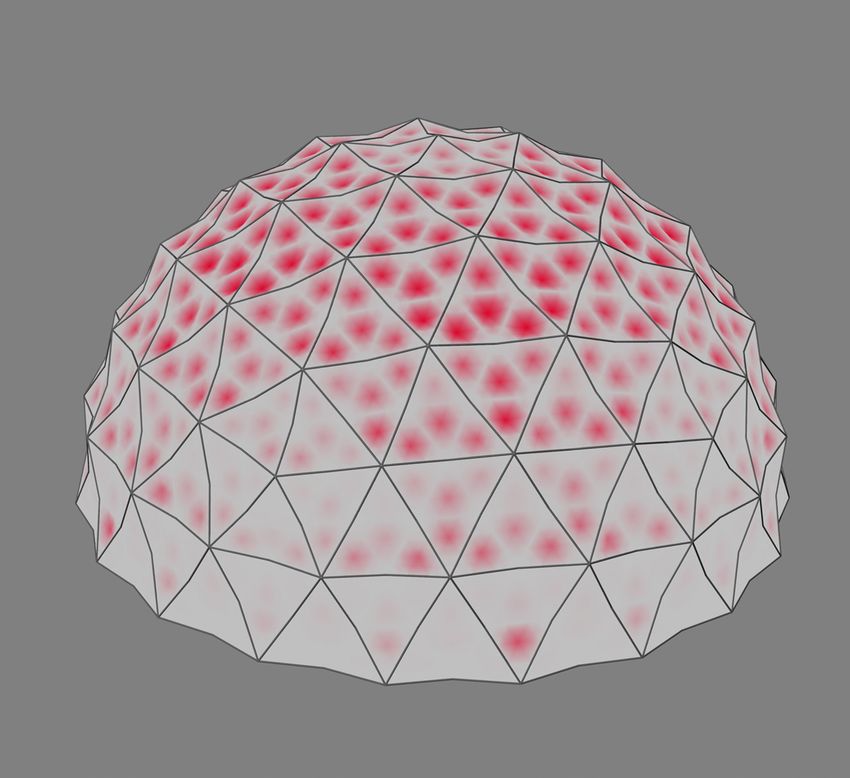
Data-driven design of deployable structures |   247

of the double layer grid. Angulated scissors are a panto- table and there is no differentiation between air inflated
graphic subtype for the single-layer grids. In the end, masts and air-supported structures. Stevenson classifies different
and arches are pantographic subtypes of spines. Consid- types of scissors. They are part of the “deploy” and “re-
ering the kinetic division, all pantographs are under the tract” category considering the physical transformation.
category of rigid links.                                       The diversity of the shapes that the scissors can form can
     Korkmaz created the next classification in 2004 [20]. It be seen through the fact that they are present in all subcat-
was focused on the deployable structures applied in archi- egories considering the classification of position in space
tecture. The definition by Fox and Yeh served as the initial and direction of transformation.
point for classification. They stated that kinetic architec-       Del Grosso and Basso started their classification from
ture comprises buildings, or components, with variable 2013 by referencing Hanaor and Levy’s table. Their work is
location and mobility in space and/or variable configura- different because of the inserting structures not mentioned
tion and geometry. This brings the concept of “time” as the earlier by other authors: compliant mechanisms under de-
crucial parameter for categorization. Because of this, the formable structures and morphing truss structures under
two initial classes are: buildings with variable geometry or rigid link structures. Following the approach of Hanaor
movement and buildings with variable location or mobility. and Levy, Del Grosso and Basso also classify scissor mech-
Prof. Korkmaz introduces pantographs as bar structures. anisms under the rigid links category [1].
In the general classification of structures, they are under        And the most recent classification comes from architect
buildings with rigid form as the part of the buildings with Esther Rivas Adrover in 2015 [23]. Although his book Deploy-
variable geometry or movement.                                 able structures is not peer-reviewed, his work is extensive.
     Classification by Schaeffer and Vogt [21] was published As the first level of division, it is taken the way on which
in 2010. It starts from differentiating movement of rigid the deployable structures are developed: one category are
materials and movement of deformable ones. On the next those based on structural components of the deployable
level, for the rigid material structures, the division was mechanisms (Structural Components), while the other are
done based on the type of the movement (rotational, trans- the structures inspired by other sources (Generative Tech-
lational or combination of the two). Deformable material nique). The first class is later subdivided to rigid deployable
structures are classified considering whether they are plas- components, deformable deployable components, flexible
tic or elastic.                                                deployables and combined deployables. The second class
     Stevenson created the next classification in a chrono- was subdivided on where does the inspiration for the struc-
logical view. It was done in 2011. Differentiation among ture comes from, so it contains origami paper pleat and
structures is two dimensional [22]. The classification ob- biomimetics. In this classification, the scissors show up
serves operations of the single parts in relation to the move- as the rigid structural components, under the category of
ment of the whole structure. The author is not using a ma- lattice work.
terial to define classes in the division, focusing instead on      As it can be noted, the scissors are one of the structures
the transformations: deforming, folding, deploying, retract- present from the first comprehensive classification and dur-
ing, sliding and revolving. Considering the issues in this ing all other versions. The system that pantographs use is
approach, pneumatic structures were not included in the known as the lazy tong system. The basic unit of the sys-

Figure 11: Classification by Del Grosso and Basso from 2013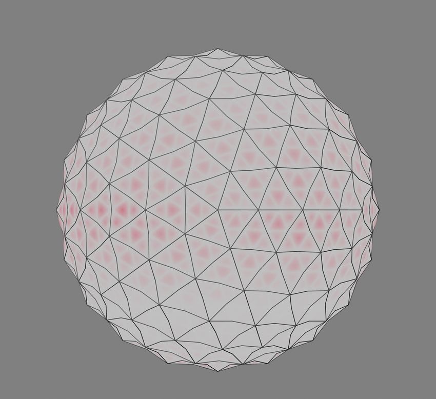
248 | M. Dragoljevic et al.

Figure 12: Classification by Rivas Adrover from 2015
Data-driven design of deployable structures |         249

Table 1: Evaluation of the double layer pantographic grids by Hanaor and Levy

Criteria                                          Evaluation
Design – Architectural flexibility                Flexible modular design is readily applicable. Large areas can be covered with relatively
                                                  small modules connected on site.
Component uniformity                              High component uniformity can be maintained, although doubly curved surfaces may re-
                                                  quire some variation in unit cell dimension.
Storage and transport – Stowed compactness        The structure folds to a compact bunch of bars. Compatible folding of the membrane cover-
                                                  ing needs to be considered.
Weight                                            Structural eflciency is medium to low, depending on the surface geometry, constituent
                                                  units and bracing.
Maintenance (wear & tear)                         Repeated deployment may cause significant wear and tear to the membrane and to connec-
                                                  tions.
Site inputs – Site preparation                    Generally, self-supporting configurations can be designed, requiring minimal foundation
                                                  and site preparation.
Connections                                       Degree of deployability is relatively high. Site connections involve connection of deployable
                                                  modules and addition of bracing elements.
Complexity / reliability                          Medium mechanical complexity. Articulated joints and hinges are relatively simple25. Hu-
                                                  man assistance in deployment is usually required.
Auxiliary equipment                               No auxiliary equipment is required other than relatively light lifting equipment to assist in
                                                  deployment and folding.

Table 2: Inclusion of the scissor structures, Zegiler’s dome and dome in the general sense in the classifications over the years

                       Merchan       Gantes     Pellegrino      Hanaor     Korkmaz      Schaeffer     Stevenson      Del Grosso        Rivas
                        (1987)       (2001)      (2001)        and Levy     (2004)      and Vogt        (2011)       and Basso        Adrover
                                                                (2001)                   (2010)                        (2013)         (2015)
Scissor structures     included      included    included      Included    included     included       included       included       included
Zeigler’s dome         included      included    included
Dome                                                                       included     included       included       included       included

tem is called a scissor-like element (SLE). It is made out of use, so besides the use of the minimum acceptable cross-
two bars and a joint that is connecting them [3]. These ele- sections the covering membrane encloses the maximum
ments can be added to each other to form parallel or curved possible volume.
systems. However, these structures require additional stabi-        This paper aims to examine the possibilities of the use
lizing elements like cables or other locking devices [10]. The of Grasshopper with Karamba in the process of optimization
other option in stabilizing is adding the internal layer of of scissor structures. The presented procedure could be
SLEs and the creation of the double-layer grid. In their work, used as a useful design tool in the early design stage.
Hanaor and Levy evaluated the double layer pantographic
grids based on their predefined criteria for deployable struc-
tures.
      The other thing to notice is that although the Zeigler’s
                                                               2 Methods
dome as a typology is present in the earliest classifications,
                                                               For enabling better control over the design process, it is
the recent ones are not focusing on it. Zeigler’s dome is the
                                                               used parametric design software Grasshopper with struc-
first example of a dome structure done with the double layer
                                                               tural calculations plug-in Karamba. The base 3D modeling
grid of pantographs. It is patented in the 1977 year [24]. The
                                                               software within which they work is Rhinoceros 3D. Thanks
reason could be the structural inefficiency of the first ver-
                                                               to this approach, the whole early-stage process of design
sions of the dome. The problems were coming from residual
                                                               is parametrized and gives full control to the designer. The
stress and bending of the elements. Considering the gen-
                                                               design process is divided into two parts: the first allows
eral shape, the dome (defined as a semi-sphere) keeps the
                                                               the parametrized control over the dimensions, shape, and
high efficiency of the sphere considering the surface area
                                                               subdivision of the general structure and the second one
to volume ratio. That means that the biggest volume can be
                                                               which performs structural calculations and confirms the
enclosed with the minimum surface. This property is in line
                                                               stability of the construction and resistance of the materials.
with the intention of the algorithm to optimize the material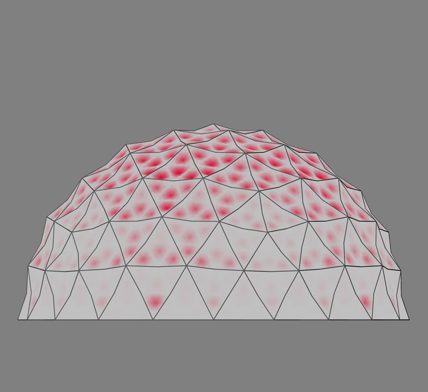
250 | M. Dragoljevic et al.
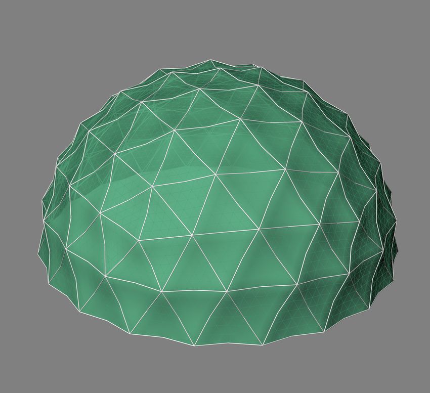
As already mentioned, the sample for testing the al-
gorithm is selected Zeigler’s dome. In the first part of
the algorithm, the properties of the geodome are defined.
For generating the initial structure, it is needed the ra-
dius, class (icosahedron/octahedron/tetrahedron) and fre-
quency (level of the division of the geodome). In the follow-
ing steps, the lines of geodome are transformed into a scis-
sor structure. A double structure is used because a single (a) (b)
layer dome does not have structural stability. This scissor
structure is used for defining the rodes and the covering
membrane. This part of the algorithm provides information
about the weight, volume and area of the structure. Also,
the length of the rodes can be checked in this step.
The second part of the algorithm is focused on struc-
tural calculations. The plug-in Karamba requires the spe-
(c) (d)
cially defined model – adjusted to its specifications and
limitations. This is a prerequisite for the use of any FEA
software [25]. In terms of modeling geometry, it is needed
to define the membrane as the mesh surface and the rods
as straight lines. Karamba uses the mesh to define a “shell”
element and the lines for the “beam” ones.
The main challenge of this approach is in the differ-
ence in the algorithms used for the membrane and the rods.
(e) (f)
Karamba allows the use of an algorithm for large deforma-
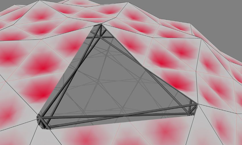
tions in the cases where elements have small dimensions Figure 13: a) Schematic view of a single field of the dome: the green
– as in the case of the covering membrane (whose thick- mesh is a membrane envelope and white tubes are the poles, b)
ness is significantly less compared to other dimensions). Blue points which are mesh vertices on the poles, observed as
support points for the membrane mesh, c) Load applied on the
However, rods are going through the deformation defined
membrane mesh with shown support points, d) Resistant forces
by the first-order theory for small deformations. Because at the support points, e) Equilibrium of the forces at the support
of this, it is needed to calculate the elements separately. points, f) Forces obtained from the equilibrium state for the support
However, this leaves the question of the load transfer from points that load the poles
one element to another.
The classical linear theory of elasticity is used for small
large deformation. The algorithm allows obtaining the re-
displacements of the deformable body. This means that the
sisting forces at supports. These forces are the opposite
positions of the points in deformed state are close to their
vectors compared to the loads that the membrane transfer
initial positions. However, in large deformation analysis,
to the rods. Thanks to this, the loads applied to the rods are
the domain of the body is changing continuously, as well as
defined and applied within the algorithm for the first-order
its boundary conditions and the external loads [26]. For the
theory deformation. For the rods system, support points
point to reach its final position at the moment t it is needed
are nodes on the ground.
to pass through different positions in time, starting from
The application of wind and snow loads is based on
0 and going through ∆t, 2∆t, 3∆t, etc. These positions are
Eurocode regulation EN 13782. However, the wind load is
obtained through incremental method of the analysis. With
adjusted to the dome structure which is not covered in detail
the algorithm based on large deformations theory, deform-
in the given document. For this is used regulation EN 1991-1-
ing body is evaluated in equilibrium positions for every
4. The coefficients for wind forces are included accordingly.
given moment. Moreover, every next moment is calculated
Materials are defined in the algorithm as well. For the
in relation to the previous one and this process is repeated
rods, it is used Steel Q235-B (S235JR), while for the mem-
until the final state of the body is not reached.
brane PVC Extruded. The important properties are given in
Since the membrane is the most external element, the
the table below (in the units used within the algorithm).
snow or wind is applying force directly to it. The membrane
The next part of the calculations is dedicated to bend-
as the element is supported along the rod lines. They are
ing moment resistance verification. It is done through a
defined as supports within the algorithm for the membraneData-driven design of deployable structures | 251
Table 3: Properties of the materials used for the structure
Material Steel Q235-B (S235JR) Extruded PVC
Young’s modulus of elasticity 20 000 kN/cm2 280 kN/cm2
Shear modulus (taken as approximately 3/8 of Young’s modulus) 7500 kN/cm2 105 kN/cm2
Specific weight 77.15 kN/m3 13.63 kN/m3
Yield strength 103.4 kN/m2 8.14 kN/m2
comparison of the maximum bending moment that the 3. Maximizing the cross-section resistance to the bend-
cross-section can resist and the maximum cross-section ing moment
that is generated within the structure. The plastic section
As the variables are used:
modulus needs to be calculated first and then using it, the
maximum bending moment that poles can resist. Formulas 1. Frequency of the structure (number of division fields
are the following ones: within the dome)
2. Poles cross-section – diameter and thickness
D3 − d3
W= Because of the 3 optimization objectives, it is possi-
6
ble to use the 3-axis space to represent potential solutions.
Thanks to this approach, it is possible for the decision-
W · fd
M c, Rd = maker to analyze potential solutions and select the one
Y M0
which is appropriate considering the production capaci-
Where ties.
– D is the external diameter of the pole
– d is the internal diameter of the pole
– YM0 = 1.1 and represents a partial factor for the resis- 3 Results
tance of cross-sections
– f d is the minimum yield strength and for the used The tested structure is an icosahedron. The initial dimen-
material (steel Q235-B) equals to 235 N/mm2 sions of the elements are the following:
The final part of the work is multivariable and multiob- – Poles: Diameter = 3 cm; Thickness = 0.5 cm
jective optimization. For this task, it used plugin Octopus. – Membrane: Thickness = 0.45 mm
The objectives of optimization are:
1. Minimizing displacement
2. Minimizing the weight of the structure
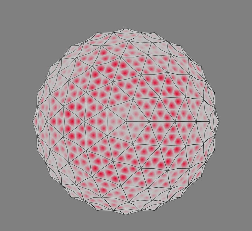
(a) (b)
Figure 14: a) Initial dome membrane model; b) Initial scissor structure dome252 | M. Dragoljevic et al.
(a) (b) (c)
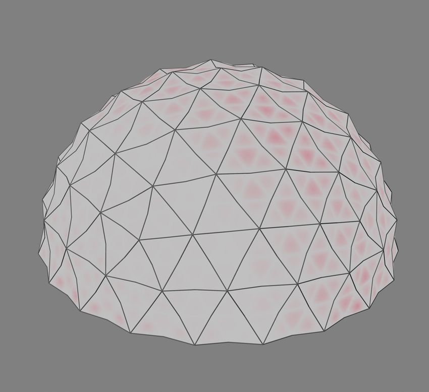
Figure 15: Fabric under the snow load (1.5 kN/m2 ); a) 3D view, b) Side view, c) Top view. Maximum displacement: 27.67 cm
(a) (b) (c)
Figure 16: Pole structure under the snow load (1.5 kN/m2 ). a) 3D view, b) Side view, c) Top view. Maximum displacement: 27.30 cm
3.1 Snow load the load values. Standard wind load for Milan by the EN
1991-1-4 equals 0.39 kN/m2 .
The first load case is the snow load. As the relevant stan-
dard, it is used Eurocode EN 1991-1-3. The selected location
is Milan, Italy. The website www.dlubal.com allows auto- 3.3 Multiobjective optimization
matic calculations of the snow and wind loads by the given
standard for locations in different countries. Standard snow Since the generated displacement and bending moment
load for Milan by the EN 1991-1-3 equals 1.5 kN/m2 . is bigger for the snow load, this case is used for structural
optimization. The optimization includes multiple objec-
tives and multiple variables. Considering the objectives, it
3.2 Wind load is important to minimize displacement and the weight of
the structure, while the acceptable bending moment for the
Wind load is the second load case. Again, as the relevant cross-section has to be bigger than the maximum generated
standard, it is used Eurocode EN 1991-1-4. The selected lo- bending moment within the structure – for this condition, it
cation is again Milan, Italy and the same source is used for is also better if this difference is bigger, but it is not decisive.Data-driven design of deployable structures | 253
(a) (b) (c)
Figure 17: Fabric under the wind load (0.39 kN/m2 ). a) 3D view, b) Side view, c) Top view. Maximum displacement: 12.52 cm
(a) (b) (c)
Figure 18: Pole structure under the wind load (0.39 kN/m2 ). a) 3D view, b) Side view, c) Top view. Maximum displacement: 3.38 cm
On the graph below, these 3 values are shown as the Considering the variables, there are cross-section (as
axes: diameter and the pole wall thickness) and frequency of the
geodome (number of subdivisions). By the Grasshopper
– Displacement [cm]
plug-in Octopus, they are not shown on the graph, but in
– Weight [kg]
the attached Table 4 there are values of variables for all
– M diff [kNm] – which is the difference between the
generated solutions.
maximum bending moment that the cross-section
Considering the comparison of the design options and
can resist and the maximum bending moment gener-
the values they generate, their impact is defined as equal.
ated by the load
This means that all the parameters are equally weighted.
In the case of the third objective (moment difference), In this case, different functions of linear standardization
any solution where the resisting moment is smaller than can be applied. Below in Table 5 are presented functions in
the generated one has to be eliminated, so all the solution the case of the maximization of the solution.
where this difference: Generated M – Resisting M is bigger If the Row maximum linear standardization is applied
than 0 are eliminated. Thanks to this, all the solutions rep- with equally weighted parameters, each set of values can
resented with the points on the graph are acceptable and
can be used for the selection of the most suitable one.254 | M. Dragoljevic et al.
Table 4: Input and output values obtained through the process of optimization (part of the data from the attachment)
Frequency Diameter [cm] Thickness [cm] Displacement Weight [kg] Bending moment difference
[cm] [kNm]
4 5.7 2.70 1.89 36433 −3.39
10 5.1 2.55 0.38 74918 −2.03
12 5.4 2.45 0.25 102053 −3.38
10 4.6 1.60 0.52 55428 −0.96
4 5.2 1.05 2.99 19817 −0.89
4 5.0 2.10 3.09 27509 −1.32
6 4.8 1.50 1.08 33494 −1.92
10 5.7 0.95 0.36 52137 −2.08
10 5.9 2.75 0.25 99646 −4.23
8 5.3 0.80 0.63 32810 −1.43
8 4.5 2.25 0.83 45945 −1.23
8 5.1 1.10 0.62 39995 −1.76
4 4.7 1.65 3.92 22814 −0.53
8 5.2 2.05 0.54 58474 −2.73
8 5.7 1.95 0.41 66153 −4.00
Table 5: Functions of linear standardization
Standardization Function
x
Row maximum
x max
(x − x min.id. )
Ideal value
(x max.id. − x min.id. )
x
Average value
x mean
(x − x min.row )
Interval standardization
(x max.row − x min.row )
x
Additive constraint ∑︀
x row
x
Vector normalization √
x2
mum [27]:
n
∑︁ xi
Figure 19: Octopus graph of multiobjective optimization Ci =
x min
1
be awarded with the sum of row maximums: Thanks to this, Table 4 can be transformed to Table 6:
n
∑︁ xi
Ci =
x max
1
However, in this case, the solutions should be minimized,
so every solution needs to be compared to the row mini-Data-driven design of deployable structures | 255
Table 6: Sum of equally-weighted row minimum standardizations
Frequency Diameter Thickness Ci
[cm] [cm]
4 5.7 2.70 10.20
10 5.1 2.55 5.78
12 5.4 2.45 6.95
10 4.6 1.60 5.10
4 5.2 1.05 13.17
Figure 20: The shape of the membrane under the load
4 5.0 2.10 14.06
6 4.8 1.50 6.46
10 5.7 0.95 4.56
10 5.9 2.75 7.03
8 5.3 0.80 4.51
8 4.5 2.25 5.93
8 5.1 1.10 4.91
4 4.7 1.65 16.96
8 5.2 2.05 5.76
8 5.7 1.95 5.92 Figure 21: Increased structural stiffness of the folded edges (com-
pared to the same material in the flat form) in the Miura origami
pattern [28]
4 Discussion
of Miura origami pattern for increasing the stiffness of the
surface.
Considering the obtained results, two areas need to be fur-
Further research could focus on physical testing at least
ther discussed: deformation of the membrane and the opti-
a single field to understand does the folding lines provide
mization process for the poles.
the greater stiffness and how much if they do. The results
could be compared with the virtual simulation.
4.1 Membrane deformation analysis
As already noted, because the membrane is done of thin
4.2 The optimization process for the poles
material, it was necessary to utilize a Large deformation
As already explained, the final outcome for the poles struc-
theory algorithm. This algorithm is adding load increments
ture is the optimization process. Since the production and
that are scaled to 1/number of increments. For the given
construction of a pantograph dome include making many
case, the number of increments is 1000.
However, during the application of the load, the mem-
brane triangular field gets the shape of the underlying pole
structure. Since the triangular field is formed by the scissor
structures, the triangle does not have flat edges, but they
are divided into two inclined parts. This causes the mem-
brane to be divided into 4 small triangular fields (as seen
in Figure 20). This creates folding lines within the same
triangular field, which later impact the algorithm. The in-
terpretation of the algorithm and the calculation software
is that these folding lines are more resistant to deformation,
therefore they remain less deformed.
This means that for the software, the folded mem-
brane behaves similar to origami patterns that are already
adopted as a method to strengthen the structure. On the
Figure 22: Application of MRA with different number of itera-
Figure 21 below, it is represented the research in the use tions [29]256 | M. Dragoljevic et al.
Table 7: Maximum nodal displacement for different dimensions of the dome
Frequency Diameter Thickness Maximum Maximum Difference Maximum Maximum Difference
[cm] [cm] nodal nodal [%] rotation angle rotation angle [%]
displacement displacement of a node of a node
(II order (I order (II order (I order
theory) [cm] theory) [cm] theory) [rad] theory) [rad]
4 5.7 2.70 1.95 1.89 0.03 0.013 0.014 0.08
4 5.2 1.05 3.17 2.99 0.06 0.022 0.021 0.05
4 5.0 2.10 3.36 3.09 0.09 0.024 0.022 0.09
6 4.8 1.50 1.24 1.08 0.15 0.012 0.011 0.09
4 4.7 1.65 4.48 3.92 0.14 0.032 0.028 0.14
6 5.2 2.60 0.91 0.82 0.11 0.009 0.008 0.13
6 4.4 2.20 1.63 1.35 0.21 0.016 0.013 0.23
6 4.3 0.65 2.63 1.98 0.33 0.026 0.020 0.30
4 5.6 1.15 2.32 2.25 0.03 0.017 0.016 0.06
6 4.1 2.05 2.13 1.67 0.28 0.021 0.017 0.24
6 4.6 0.70 1.97 1.59 0.24 0.020 0.016 0.25
6 3.5 1.75 4.28 2.69 0.59 0.044 0.027 0.63
6 3.9 0.85 3.22 2.27 0.42 0.033 0.022 0.50
4 5.3 1.00 3.01 2.86 0.05 0.022 0.020 0.10
6 3.8 1.90 2.92 2.10 0.39 0.030 0.021 0.43
4 5.9 2.55 1.71 1.67 0.02 0.012 0.012 0.00
4 5.0 2.40 3.36 3.09 0.09 0.024 0.022 0.09
6 6.0 0.70 0.85 0.78 0.09 0.009 0.008 0.13
6 4.1 2.05 2.13 1.67 0.28 0.021 0.017 0.24
4 5.2 1.20 3.03 2.87 0.06 0.022 0.020 0.10
6 5.1 0.70 1.4 1.20 0.17 0.014 0.012 0.17
4 4.7 1.45 4.52 3.97 0.14 0.032 0.028 0.14
4 5.1 2.55 3.09 2.87 0.08 0.022 0.020 0.10
6 5.0 1.15 1.16 1.15 0.01 0.012 0.010 0.20
6 4.6 0.80 1.81 1.48 0.22 0.018 0.015 0.20
6 4.7 1.85 1.3 1.12 0.16 0.013 0.011 0.18
4 5.1 2.55 3.09 2.87 0.08 0.022 0.020 0.10
6 4.7 0.90 1.58 1.33 0.19 0.016 0.013 0.23
6 4.1 2.05 2.13 1.67 0.28 0.021 0.017 0.24
Avg. 0.17 Avg. 0.19
difference difference
decisions, the multiobjective optimization does not bring sort data and select the more suitable ones for production
a single solution that is better than the others. Instead, it and construction.
creates a matrix of connected starting variables and final Further research could go in the direction of checking
values which can be evaluated by the decision-maker. the behavior of the real scissor models and comparison
In this case, in Table 4, there are inputs frequency, di- with the virtually obtained data.
ameter and thickness for the structure and results general The other important question for the optimization of
displacement, the weight of the structure and bending mo- the poles is their stability. Considering the instability of
ment difference (maximum generated bending moment – the model, use of the linear approach (first-order theory of
the maximum bending moment which the cross-section deformation) does not provide the response on the stability
can resist). Bending difference is always set to be negative of the system. The stability could be controlled through the
because the maximum generated bending moment has to two additional procedures.
be smaller than the bending moment which cross-section The first useful procedure for this case could be the
can resist. multi-body rope approach. By virtually loading nodes
Thanks to the presented information, the decision- within the structural system, it is possible to bring it to the
maker can give “weight” to each result and compare or stable configuration. However, the form of the deployable
structures is determined by the deployability mechanismData-driven design of deployable structures | 257
as well, so perhaps the results cannot reach the perfectly
optimized configuration as in the case with the ropes. There-
References
fore, the mechanism design should be integrated with MRA [1] Del Grosso A, Basso P. Deployable Structures. Advances in Sci-
for the best results. ence and Technology. 2012;83:122–31.
Considering the second approach for checking the in- [2] Jensen FV. Concepts for retractable roof structures. PhD thesis;
stability of the system, it can be done by applying the 2005.
second-order theory algorithm and the comparison of the [3] De Temmerman N. Design and analysis of deployable bar struc-
tures for mobile architectural applications. Vrije Universiteit
nodal displacement with the results obtained through first-
Brussel; 2007.
order theory analysis. As already described in one of the [4] Zuk W, Clark RH. Kinetic architecture. Van Nostrand Reinhold
previous chapters, the second order theory is based on in- Company; 1970.
cremental application of the loads on the structure. It takes [5] Rowan J. Progressive architecture. Philip H. Hubbard; 1968.
the structure through the intermediate states until reaching [6] Escrig F. Expandable space structures. Int J Space Struct.
1985;1(2):79–91.
the final one. The final position of the structure is therefore
[7] Forster B. Cable and membrane roofs – a historical survey. Struct
the stable configuration considering the given loads. Eng Rev. 1994;6:145–74.
When applying this algorithm on the initial structure [8] Mollaert M. Retractable membrane roofs. WIT Transactions on
(frequency of the geodome = 4; diameter of the pole = 3cm, the Built Environment. WIT Press. 1996;21:407–17.
wall thickness = 0.5cm), there is an issue of buckling in the [9] Friedman N. Investigation of highly flexible, deployable struc-
case of the snow load. In this case, the compressive normal tures: review, modelling, control, experiments and application.
Budapest University of Technology and Economics; 2001.
forces are too big and it causes buckling of the structural
[10] Doroftei I, Doroftei I–A. Deployable structures for architectural
system. As the result, the algorithm is unable to calculate applications – a short review. Applied Mechanics and Materials.
the behavior of the structure. In further research, with the 2014; 658: 233–40.
changes in the diameter and wall thickness and through [11] Puig L, Barton A, Rando N. A review on large deployable struc-
the application of the same approach, it is possible to mini- tures for astrophysics missions. Acta Astronautica. 2010; 67:
12–26.
mize the nodal displacement values. Below is Table 7 with
[12] Ramzy N, Fayed H. Kinetic systems in architecture: new approach
the maximum nodal displacement for different values of for environmental control systems and contextsensitive build-
the diameter and wall thickness of the poles. Because of ings. Sustain Cities Soc. 2011;1:170–7.
the complexity of the system, the II order theory analysis is [13] Santiago–Prowald J, Baier H. Advances in deployable struc-
performed for frequencies 4 and 6. Also, there is an issue of tures and surfaces for large apertures in space. CEAS Space
the system undergoing buckling (as the initial dimensions J. 2013;5:89–115.
[14] Merchan CHH. Deployable structures. Massachusetts Institute
of the given system), so the procedure of looking for a mini-
of Technology; 1987.
mum requires a second check is the system under buckling [15] Kaveh A, Davaran A. Analysis of pantograph foldable structures.
or not. Comp & Struct. 1996;59(1):131–40.
As it can be seen in the upper table the average dif- [16] Gantes CJ. Deployable structures: analysis and design. WIT Press;
ference in displacement between two approaches (I and II 2001.
[17] Fenci GE, Currie NG. Deployable structures classification: A re-
order theory) is 17% for maximum nodal displacement and
view. Int J Space Struct. 2017;32(2):112–30.
19% for the rotation angle. [18] Pellegrino S. (eds) Deployable Structures. International Centre
for Mechanical Sciences (Courses and Lectures). Springer; 2001.
Funding information: The authors state no funding in- [19] Hanaor A, Levy, R. Evaluation of Deployable Structures for Space
volved. Enclosures. Int J Space Struct. 2001;16:211–29.
[20] Korkmaz K. An analytical study of the design potentials in kinetic
architecture. İzmir Institute of Technology; 2004.
Author contributions: All authors have accepted responsi-
[21] Schaeffer O, Vogt MM, Scheuermann A. MOVE: architecture in
bility for the entire content of this manuscript and approved motion – dynamic components and elements. Birkhäuser. 2010.
its submission. [22] Stevenson CM. Morphological principles: current kinetic archi-
tectural structures. Adaptive Architecture. 2011; 1–12.
Conflict of interest: The authors state no conflict of inter- [23] Adrover ER. Deployable Structures. Laurence King Publishing.
2015.
est.
[24] Zeigler TR. Collapsible self–supporting structure. Patent
3,968,808. 1976.
[25] Preisinger C, Moritz H. Karamba – A Toolkit for Parametric Struc-
tural Design. Struct Eng Int. 2014;24(2):217–21.
[26] Gomez Botero M. Finite element formulation for large displace-
ment analysis. Universidad EAFIT; 2009.258 | M. Dragoljevic et al.
[27] Lacidogna G, Scaramozzino D, Carpinteri A. Optimization of di- [29] Manuello A. Multi–body rope approach for grid shells: Form–
agrid geometry based on the desirability function approach. finding and imperfection sensitivity. Eng Struct. 2020; 221.
Curved Layered Struct. 2020;7:139–52.
[28] Wei ZY, Guo ZV, Dudite L, Liang HY, Mahadevan L. Geomet-
ric Mechanics of Periodic Pleated Origami. Phys Rev Lett.
2013;110:215501.You can also read