Combined Naïve Bayesian, Chemical Fingerprints and Molecular Docking Classifiers to Model and Predict Androgen Receptor Binding Data for ...
←
→
Page content transcription
If your browser does not render page correctly, please read the page content below
International Journal of
               Molecular Sciences

Article
Combined Naïve Bayesian, Chemical Fingerprints and
Molecular Docking Classifiers to Model and Predict Androgen
Receptor Binding Data for Environmentally- and
Health-Sensitive Substances
Alfonso T. García-Sosa *                  and Uko Maran *

                                           Institute of Chemistry, University of Tartu, Ravila 14a, 50411 Tartu, Estonia
                                           * Correspondence: alfonsog@ut.ee (A.T.G.-S.); uko.maran@ut.ee (U.M.); Tel.: +372-737-5270 (A.T.G.-S.);
                                             +372-737-525 (U.M.)

                                           Abstract: Many chemicals that enter the environment, food chain, and the human body can disrupt
                                           androgen-dependent pathways and mimic hormones and therefore, may be responsible for multiple
                                           diseases from reproductive to tumor. Thus, modeling and predicting androgen receptor activity is
                                           an important area of research. The aim of the current study was to find a method or combination of
                                           methods to predict compounds that can bind to and/or disrupt the androgen receptor, and thereby
                                           guide decision making and further analysis. A stepwise procedure proceeded from analysis of protein
                                           structures from human, chimp, and rat, followed by docking and subsequent ligand, and statistics
                                 based techniques that improved classification gradually. The best methods used multivariate logistic
                                    regression of combinations of chimpanzee protein structural docking scores, extended connectivity
Citation: García-Sosa, A.T.; Maran,        fingerprints, and naïve Bayesians of known binders and non-binders. Combination or consensus
U. Combined Naïve Bayesian,                methods included data from a variety of procedures to improve the final model accuracy.
Chemical Fingerprints and Molecular
Docking Classifiers to Model and           Keywords: androgen receptor; bayesian; multivariate logistic regression; chemical fingerprints; ecfp;
Predict Androgen Receptor Binding          docking; toxicity; human; chimp; rat
Data for Environmentally- and
Health-Sensitive Substances. Int. J.
Mol. Sci. 2021, 22, 6695. https://
doi.org/10.3390/ijms22136695
                                           1. Introduction
Academic Editor: Bono Lučić
                                                Concern has been rising due to the fact that many environmental factors can modulate
                                           the androgen receptor (AR) pathway: agricultural and industrial chemicals, pharmaco-
Received: 6 March 2021                     logical drugs and chemotherapeutics, aging, hyperthermia, and chronic infection, alcohol,
Accepted: 20 June 2021                     tobacco, and other drugs [1–4]. These chemical agents enter the waterways, food chain,
Published: 22 June 2021                    and affect other environments. In vivo rodent models are one way to try to elucidate the
                                           exact roles of AR in reproduction and the molecular mechanism of AR modulation in
Publisher’s Note: MDPI stays neutral       reproductive health [1–4]. Modulation of the AR has multiple biological effects on species
with regard to jurisdictional claims in    in the environment, on health, and diseases. These include important roles in the develop-
published maps and institutional affil-    ment and maintenance of reproductive [5], musculoskeletal [6,7], cardiovascular [8–10],
iations.                                   immune [11,12], nervous [13–15], and hematopoietic [16,17] systems. The AR has also been
                                           shown to be associated with the development of prostate [18], breast [19,20], bladder [21],
                                           liver [22], kidney [23], and lung [24] tumors [25]. Chemicals that mimic hormones can
                                           cause abnormalities and undesirable effects in the hormonal system, which in turn can
Copyright: © 2021 by the authors.          lead to many of the aforementioned diseases. However, the number of synthesized and
Licensee MDPI, Basel, Switzerland.         commercially produced chemicals is constantly increasing, resulting in more of them reach-
This article is an open access article     ing the environment, the food chain, and eventually the human body. The compounds of
distributed under the terms and            most concern are those that may disrupt hormone-receptor binding in the body, or prevent
conditions of the Creative Commons         other interactions that are responsible for metabolism, transport, or synthesis of substances,
Attribution (CC BY) license (https://      such as endocrine disrupting chemicals (e.g., disrupting the hormonal system) [5,26]. For
creativecommons.org/licenses/by/           example, AR binding compounds, or those that interfere with androgen-dependent path-
4.0/).

Int. J. Mol. Sci. 2021, 22, 6695. https://doi.org/10.3390/ijms22136695                                            https://www.mdpi.com/journal/ijms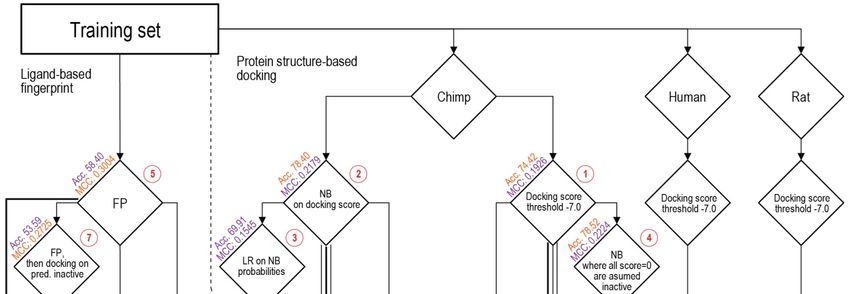
Int. J. Mol. Sci. 2021, 22, 6695                                                                                           2 of 13

                                   ways, can be responsible for increased infertility and decreased sperm counts [27], prostate
                                   cancer, testicular dysgenesis syndrome, among others [28,29].
                                         AR pathway interactions may or may not be due to ligand binding on the androgen
                                   receptor [30]. The former, ligand-dependent, are in turn divided into two: the androgen
                                   molecule/AR pathway event involves DNA (so-called genomic); or where interaction with
                                   DNA does not occur (so-called non-genomic) [30]. These AR-activity related interactions
                                   can be modeled with a variety of computational approaches [31]. Different techniques
                                   can be used to predict the binding of compounds to a receptor, or to infer the binding or
                                   activity of a compound. If a protein structure is available, structure-based methods may
                                   be used [32–34]. Androgen receptor binding has been modeled for toxicology, but also for
                                   drug design [32]. Ligand-based methods that use statistical approaches are an alternative
                                   for modeling androgen receptor binding without using the structure of the protein, mostly
                                   QSAR methods, mainly dealing with specific series of compounds, but also with general
                                   series of compounds [31,35–39]. Even if there is a wealth of data on the androgen receptor,
                                   it is generally recognized that this is difficult system to model [31], as well as expensive
                                   and difficult to assay in vivo, in human, and other model systems.
                                         Modeling opportunities were made available recently via the US Environmental
                                   Protection Agency (EPA) Collaborative Modeling Project for Androgen Receptor Activity
                                   (CoMPARA) [40]. The CoMPARA project used data from the integrated experimental
                                   and computational approach that combined data from 11 ToxCast and Tox21 in vitro high
                                   throughput screening (HTS) assays measuring activity at multiple points along the AR
                                   pathway: receptor-binding, coregulator recruitment, chromatin-binding of the mature
                                   transcription factor, and gene transcription [41]. Within the CoMPARA project, different
                                   modeling approaches were used by the consortium of 25 collaborating research teams to
                                   evaluate the androgenic potential of compounds, and finally, the prediction results and
                                   modelling methods were combined into a consensus [42]. A similar collaborative project
                                   was carried out previously to predict compounds with potential estrogenic activity in the
                                   Collaborative Estrogen Receptor Activity Prediction Project (CERAPP) [43].
                                         The aim of the present study was to find a method or combination of methods,
                                   including consensus modeling, to allow predicting compounds that may bind to the
                                   important AR and/or disrupt androgenic pathways, and through this pathway may cause
                                   undesired and dangerous health outcomes. These predictions, in turn, can guide decision
                                   making and further analysis of compounds. The consensus combinations are employed for
                                   molecular docking, chemical fingerprints, naïve Bayesian, and logistic regression methods.
                                   Predictions of the final model of this study were originally submitted to the CoMPARA
                                   project as one of the three modeling methods of our research group, but were not included
                                   into the overall consensus model as during the course of the CoMPARA project, a limit
                                   was set for the submissions by one research group.

                                   2. Methods
                                   2.1. Data Sets and Molecular Structures
                                        The dataset of active, i.e., binding compounds (n = 205, composed of both agonists
                                   and antagonists), and inactive (i.e., non-binding, n = 1480) compounds was obtained from
                                   the CoMPARA project website [40,41], and named training set (n = 1685, Table S1). A
                                   validation data set (n = 20, Kleinstreuer et al. [41]) with AR reference compounds included
                                   was used, that contained indication of their binding status. An evaluation data set (n = 3882,
                                   Table S2) was also provided by the CoMPARA project organizers [42] and was processed
                                   and scored with the best model trained with the training set. The status for each binding
                                   compound was reported as “Binding” in the SDF file (ToxCast_AR_Binding-2016-11-17.sdf).
                                   We considered the field “hitcall” in the SDF file that divided the compounds into “Active”
                                   and “Inactive” in order to test the procedure. This gave nactive = 453, ninactive = 3429. All
                                   chemical structures were used as the QSAR ready SMILES provided within the CoMPARA
                                   project; ‘QSAR ready’ means that salts were converted into neutral form, counterions were
                                   removed, tautomers were normalized, etc. (detailed description about datasets and their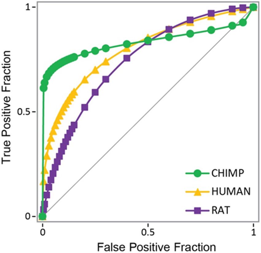
Int. J. Mol. Sci. 2021, 22, 6695                                                                                            3 of 13

                                   assembly are provided in reference [42]). Minimized 3D structures of the ligands were also
                                   prepared by the CoMPARA organizers.

                                   2.2. Molecular Docking
                                        The data provided by the CoMPARA organizers contained data including in vitro
                                   compound assays on chimp, human, and rat androgen receptors [41]. In the present work
                                   we were more interested in grouping the actives as binders, irrespective if they were either
                                   agonist or antagonist, as both classes would presumably bind to the AR. The inactive
                                   compounds (organizer definition ‘inactive’ was Activity concentration >800 µM) were
                                   taken to be non-binders. Docking was performed using Glide XP v. 2017, as contained
                                   in the Schrodinger suite [44], with conditions as described previously, [34] with the main
                                   difference of docking being performed in the orthosteric site of AR using 15 Å inner box
                                   and 40 Å outer search boxes.

                                   2.3. Protein Structures
                                        The protein structure for the androgen receptor for chimp (Pan troglodytes), human
                                   (Homo sapiens), and rat (Rattus norwegicus) species were downloaded from the PDB [45],
                                   with structure codes (resolution) 1t7r (1.4 Å), 3v49 (1.7 Å), and 3g0w (1.95 Å), respectively.
                                   These structures were selected based on the availability of a protein-ligand complex, the
                                   highest possible X-ray crystal structure resolution, and the completeness of amino acid
                                   residue sequence. The best crystal structure among these was selected as the one that gave
                                   the best separation of known binders and non-binders. Structure 1t7r contains the AR in
                                   complex with 5-alpha-dihydrotestosterone at a resolution of 1.4 Ångströms.

                                   2.4. Characterization and Comparison of Ligands
                                         Chemical fingerprints were generated using Extended Chemical Fingerprints (ECFP),
                                   a circular fingerprint as encoded by Instant JChem [46]. Distances between chemical
                                   fingerprints were calculated by Tanimoto (a.k.a. Jaccard, T) coefficient for the case of a
                                   binary fingerprint (bit string), according to Equation (1), where NA and NB are the number
                                   of bits set in the bit strings of molecules A and B, respectively, and NA&B is the number of
                                   bits that are set in both.
                                                                                      NA&B
                                                                     T ( A, B) =                                            (1)
                                                                                 NA + NB − NA&B
                                       The dissimilarity or distance between molecules is calculated according to Equation (2),
                                   where T(A, B) is the Tanimoto coefficient for molecules A and B.

                                                                       D ( A, B) = 1 − T ( A, B)                               (2)

                                   2.5. Naïve Bayesians
                                         Bayesian classifiers were calculated according to Equation (3), where µ is the mean,
                                   σ is the standard variation, and x is the independent variable, in this case the docking
                                   scores [47].
                                                                                 1      ( x − µ )2
                                                                                      −
                                                                     P( x ) = √      e 2πσ2                               (3)
                                                                                2πσ2
                                         The probabilities are calculated for both binders and non-binders and their ratio for the
                                   values calculated for a new compound determines their classification into either group, i.e.,
                                   if a probability for a compound was higher for the binding group than for the non-binding
                                   group, the compound was classified as a binder and vice versa.

                                   2.6. Multivariate Logistic Regression
                                        Multivariate logistical regression [48] was used according to Equation (4), where Pcmpd
                                   is the probability of a compound of belonging to class 1 (classified as binding), or class 0
Int. J. Mol. Sci. 2021, 22, 6695 4 of 13
(coded non-binding), based on the variables X1 . . . n that are properties of the compound
and their coefficients α1 . . . N .
e( β+α1 X1 +... αn Xn )
Pcmpd = (4)
1 + e( β+α1 X1 +... αn Xn )
The linear form of Equation (4) (logit(Y)) can have infinitely large or small values
for the dependent variable, so instead of ordinary least squares, maximum likelihood
techniques are used to maximize the value of the log likelihood (LL) function, which
indicates how likely it is to obtain the observed values of Y, given the values of the
independent variables and the parameters β, α1 , . . . , αn .
2.7. Performance Analysis
The confusion matrix is usually defined as the collection of four fields: true positives
(TP), true negatives (TN), false positives (FP), and false negatives (FN). Using these values,
common measures can be calculated that allow to evaluate the quality of a prediction,
such as specificity (SP): TN/(TN + FP), sensitivity (SE): TP/(TP + FN), accuracy (Acc.):
(TP + TN)/(TP + FP + FN + TN), and Matthews correlation coefficient (MCC). The MCC
was calculated for all procedures according to Equation (5).
TP· TN − FP· FN
MCC = p (5)
( TN + FN )·( TN + FP)·( TP + FN )·( TP + FP)
For more detailed analysis, we added several other measures: the probability that a
chemical predicted as a binder is actually a binder (PPV, Equation (6)), the probability that
a chemical predicted as a nonbinder is actually a nonbinder (NPV, Equation (7)), positive
(+LR, Equation (8)) and negative (−LR, Equation (9)) likelihood ratios [49], and modified
correct classification rate, giving higher scores for models with optimal balance between
SE and SP (BCR, Equation (10)) [50].
TP
PPV = (6)
TP + FP
TN
NPV = (7)
TN + FN
SE
+ LR = (8)
1 − SP
1 − SE
− LR = (9)
SP
SE + SP
BCR = × (1 − | SE − SP| ) (10)
2
2.8. Availability of Best Model
The numerical raw data and best classification model is provided in the QSAR Data
Bank format [51] and uploaded to the QsarDB repository [52,53]. A digital object identifier
(DOI) is assigned for the model and data [54].
3. Results
3.1. Androgen Receptor from Chimp as Model Protein
The self-docking of the known binder dihydrotestosterone into structure 1t7r gave
a strong docking score of −11.91 kcal/mol. The root-mean-square deviation (RMSD) of
atom positions between the docked pose and the initial position of the co-crystallized
ligand was 0.32 Å, indicating a good fit and small deviation from the crystal structure.
Another known binder, testosterone, also scored a strong docking score of −10.32 kcal/mol.
To widen the window for the predictions, we decided heuristically to use a (relatively3.1. Androgen Receptor from Chimp as Model Protein
The self-docking of the known binder dihydrotestosterone into structure 1t7r gave a
strong docking score of −11.91 kcal/mol. The root-mean-square deviation (RMSD) of
atom positions between the docked pose and the initial position of the co-crystallized
Int. J. Mol. Sci. 2021, 22, 6695 ligand was 0.32 Å, indicating a good fit and small deviation from the crystal structure. 5 of 13
Another known binder, testosterone, also scored a strong docking score of −10.32
kcal/mol. To widen the window for the predictions, we decided heuristically to use a
(relatively
strong) strong)
threshold threshold
value value of as
of −7 kcal/mol −7this
kcal/mol as this would
would correspond correspondtoapproxi-
approximately ligand
mately to ligand submicromolar K values. After docking the known
submicromolar Kd values. After docking the known binders and known non-binders
d binders and known to
non-binders
the to theprotein
three different three different protein
structures fromstructures from
the different the different
species, species,
the results the results
showed best
showed best
agreement withagreement with experimental
experimental values (binding values (binding
status) status)
using the chimpusing the chimp
protein pro-
structure,
tein structure,
rather than using rather
humanthanorusing humanstructures
rat protein or rat protein structures
in molecular in molecular
docking, docking, or
or a combination
of the three (Figure
a combination of the1).three
Receiver-operator curves and areacurves
(Figure 1). Receiver-operator underand the curve (AUC)
area under values
the curve
provided further
(AUC) values validation,
provided giving
further AUC values
validation, of 0.832
giving AUCfor chimp,
values 0.797 for human,
of 0.832 and
chimp, 0.797
0.744 for rat AR.
for human, and 0.744 for rat AR.
Figure1.1.Receiver-operator
Figure Receiver-operatorcurves
curvesfor
fordocking
dockingtotothe
thehuman
human(in
(inyellow),
yellow),rat
rat(in
(inpurple),
purple),and
andchimp
chimp
(in green) androgen receptor as compared to a random pick (diagonal line). Chimp AUC
(in green) androgen receptor as compared to a random pick (diagonal line). Chimp AUC = 0.832; = 0.832;
human AUC = 0.797; and rat AUC =
human AUC = 0.797; and rat AUC = 0.744. 0.744.
The chimp
The chimpdocking
dockingresults
results distribution
distribution waswas analyzed
analyzed for both
for both binding
binding and
and non-
non-binding compounds in the training set (Figure 2), showing that around
binding compounds in the training set (Figure 2), showing that around half of the com- half of the
compounds for both binding and non-binding compounds had a docking
pounds for both binding and non-binding compounds had a docking score of zero, while score of zero,
while
the thehalf
other other
washalf was indeed
indeed separated, separated, with binding
with binding compoundscompounds havingdistributed
having values values dis-
tributed
over deeperover deeper
docking docking
scores. scores.
This good This good
resolution resolution with
for compounds for compounds with a
a non-zero docking
non-zero
score docking
prompted score prompted
to search for a further to way
searchto for a further
separate way to separate
the compounds that the
did compounds
not resolve
that i.e.,
well, did those
not resolve
bindingwell, i.e., those binding
and non-binding and non-binding
compounds compounds
that had a docking that
score of had a
zero.
docking score of zero.
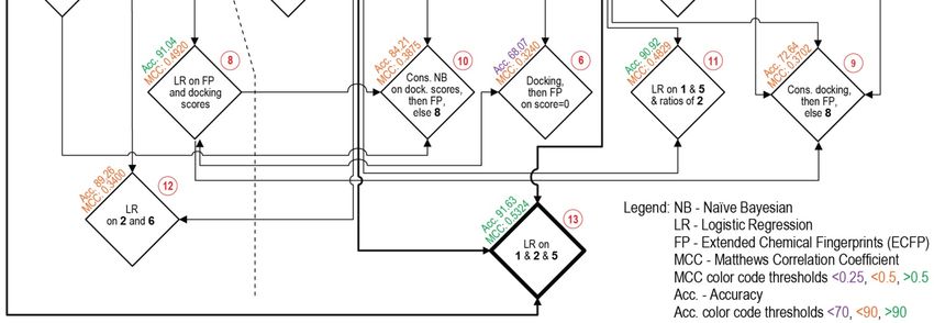
3.2. Consensus Methods for Best Performance
Subsequently, various methods and combinations thereof were applied to separate the
binding and non-binding compounds (Figure 3). For this, several different metrics were
checked for each procedure, with the Acc. and MCC as the primary metrics to guide the
improvement of the procedures. The range of MCC is from −1, total disagreement between
prediction and observation, to +1, a perfect prediction. Different procedures applied to
the training set and their sequential relationship are schematically viewed in Figure 3,
where horizontal levels from top to bottom show the complexity of combinations and path
towards the improvement of the Acc. and MCC values.Int. J. Mol. Sci. 2021, 22, 6695
Int. J. Mol. Sci. 2021, 22, 6695 6 of 13
Int. J. Mol. Sci. 2021, 22, 6695 Figure Distributions of docking scores (in kcal/mol) for bindingfor
(agonists plus(agonists 7 ofand
antagonists) 14
Figure2. 2. Distributions of docking scores (in kcal/mol) binding plus antagon
non-binding compounds for the training set against chimp protein.
non-binding compounds for the training set against chimp protein.
3.2. Consensus Methods for Best Performance
Subsequently, various methods and combinations thereof were applied to sepa
binding and non-binding compounds (Figure 3). For this, several different metr
checked for each procedure, with the Acc. and MCC as the primary metrics to g
improvement of the procedures. The range of MCC is from −1, total disagreem
tween prediction and observation, to +1, a perfect prediction. Different proced
plied to the training set and their sequential relationship are schematically vi
Figure 3, where horizontal levels from top to bottom show the complexity of c
tions and path towards the improvement of the Acc. and MCC values.
Figure
Figure 3.
3. Flowchart
Flowchart of
of the
the different
different Procedures (1–13, see
Procedures (1–13, see Section
Section 3.2
3.2 in
in text)
text) applied
applied on
on the
the training
training set.
set.
A first attempt at separation used a threshold on the docking scores in order to
classify compounds into binding and non-binding. Different values were tested, with the
best being a threshold score value of −7 kcal/mol. Compounds with scores above this
level were classified as non-binders, and scores below this level were classified as binders
(Figure 3: Procedure 1). Despite the fact that the Acc. value is relatively good, the MCCInt. J. Mol. Sci. 2021, 22, 6695 7 of 13
A first attempt at separation used a threshold on the docking scores in order to classify
compounds into binding and non-binding. Different values were tested, with the best being
a threshold score value of −7 kcal/mol. Compounds with scores above this level were
classified as non-binders, and scores below this level were classified as binders (Figure 3:
Procedure 1). Despite the fact that the Acc. value is relatively good, the MCC value is the
lowest of all the tested Procedures (Table 1).
Table 1. True positives (TP), true negatives (TN), false positives (FP), false negatives (FN), specificity (SP, %), sensitivity (SE,
%), accuracy (Acc., %), and Matthews correlation coefficient (MCC) for 13 different procedures for the training set.
Procedure TP TN FP FN SP SE Acc. MCC
1 Docking score threshold 97 1157 323 108 78.18 47.32 74.42 0.1926
2 Bayesian on scores 89 1232 248 116 83.24 43.41 78.40 0.2179
3 Logistic regression on Bayesian 100 1078 402 105 72.84 48.78 69.91 0.1545
4 Modified Bayesian 90 1233 247 115 83.31 43.90 78.52 0.2224
5 Fingerprints (ECFP) 189 795 685 16 53.72 92.20 58.40 0.3004
6 Docking scores then ECFP 169 978 502 36 66.08 82.44 68.07 0.3240
7 ECFP then docking scores 191 712 768 14 48.11 93.17 53.59 0.2725
8 Logistic regr. on docking scores and ECFP 71 1463 17 134 98.85 34.63 91.04 0.4920
9 Consensus Docking and ECFP else 8 170 1054 426 35 71.22 82.93 72.64 0.3702
10 Consensus Bayesian and ECFP else 8 117 1302 178 88 87.97 57.07 84.21 0.3875
Logistic regr. on docking scores and ECFP
11 69 1463 17 136 98.85 33.66 90.92 0.4829
and ratio of Bayesian
Logistic regression on and Bayesian avgs.
12 42 1462 18 163 98.78 20.49 89.26 0.3400
and fingerprints
Logistic regression on docking scores and
13 75 1469 11 130 99.26 36.59 91.63 0.5324
Bayesian avgs. and fingerprints
Naïve Bayesian classifiers were constructed with the docking scores of both active
(binding) and inactive (non-binding) compounds, resulting in mean values of µ = −8.91
and −5.97 kcal/mol, and standard deviations (SD) = 1.94 and 2.01, respectively. The results
of using only this classifier on its own are shown in Table 1: Procedure 2.
Procedure 3 was similar to Procedure 2, using a univariate logistic regression on the
naïve Bayesian classifier probabilities. Procedure 4 was a modification of the Bayesian clas-
sifier, in which the docking score was used as in the first procedure, reducing the number
of false positives by assuming zeroes were non-binding compounds. Both procedures did
not improve the MCC values, while giving reduced Acc. values.
The following, Procedure 5, was ligand-based and involved calculating the distance
between ECFPs for a compound and the known binders and non-binders. The smaller
the distance between the ECFPs and each group, either the average distance towards
known binders or average distance to known non-binders, would indicate the similarity
of a compound to either group. This procedure resulted in an improved separation and
therefore improved MCC at 0.3, while Acc. decreased.
Docking scores and ECFPs were used together for Procedure 6. Here, the threshold
of −7 kcal/mol was used first on the docking scores, and the compounds that registered
0 kcal/mol were then separated using ECFPs. This combination had again the effect of
improving the separation and thus, the Acc. and MCC values. Procedure 7 was similar, but
was used in the inverted order, i.e., if the ECFP predicted a non-binder, then the docking
score threshold was used. The latter procedure was not as effective as the former, giving a
lower MCC and the lowest Acc. among Procedures.
For Procedure 8, a logistic regression was used on the docking scores and difference
between ECFP distances to binders and non-binders. This improved the separation and
provided the increase in MCC to 0.492 and the second best Acc. among the procedures.
Procedure 9, used a sequence such as in Procedure 6, first docking scores, then ECFP, and
then, if a zero was still obtained, used the logistic regression in Procedure 8. Neither this,Int. J. Mol. Sci. 2021, 22, 6695 8 of 13
nor Procedure 10 were better than Procedure 8. Procedure 10 was analogous to procedure 7,
adding the logistic regression from 8 to the sequence.
Procedure 11 used a new logistic regression on the docking scores, ECFP differences,
and ratio of Bayesian predicted classifications. This resulted in better separation than 10,
an MCC to 0.4829 and third best Acc. Procedure 12 was similar to 11, but employed the
Bayesian averages instead of the ratio. However, 11 and 12 performed similarly.
Out of all the combinations, a multivariate logistical model emerged as the best per-
forming (Procedures 8 and 11). The best equation obtained was Procedure 13, represented
as Equation (11) (http://dx.doi.org/10.15152/QDB.235, accessed on 21 June 2021).
e 1
Pcmpd = = (11)
1 + eY 1 + e −Y
Y = 26.169 – 0.0175∗ChimpDockScore − 98.582∗avgDAct + 66.953∗avgDInact
+3.584∗ PAct_dockChimp – 8.594∗PInact
where
Y = 26.169 – 0.0175∗ChimpDockScore − 98.582∗avgDAct + 66.953
∗avgDInact + 3.584∗ PAct_dockChimp – 8.594∗PInact
This final model includes five descriptors: the docking score for the compound with
chimp protein (ChimpDockScore), the average of the distances to the known active (toxic)
chemicals (avgDAct ), the average of the distances to the known inactive (non-toxic) chemi-
cals (avgDInact ), the Bayesian probability value for the compound according to the distribu-
tion of known actives (toxic) compounds towards the chimp protein (PAct_dockChimp ), and
the Bayesian probability value for the compound according to the distribution of known
inactives (non-toxic) compounds towards the chimp protein (PInact ).
For Equation (11), Procedure 13 (http://dx.doi.org/10.15152/QDB.235), the best
indicator of performance was recorded by a LogLikelihood (LL) value of −407.619. The
values for true positives (TP), true negatives (TN), false positives (FP), and false negatives
(FN) were: 75, 1469, 11, and 130, respectively. SP (true negative rate) = 99.26%, SE (true
positive rate) = 36.59%, Accuracy = 91.63, the first and the last being the highest among
tested procedures. The MCC gave a value of 0.5324, which is better than random and the
best result for MCC obtained from the several options tried. Removal of 15 compounds
referred to as likely false positives [55] gave a slightly better value of MCC = 0.5364. This
procedure resulted also in the highest Accuracy value.
In more detailed analysis, NPV, PPV, +LR, −LR, and BCR statistics showed a slightly
different view of the models (Table 2). In computational toxicology, one wishes to predict
potentially harmful chemicals, minimizing FNs. This implies a classification model is
usable even if it gives a high rate of FPs (low PPVs) but a low number of FNs (high
NPVs) [56]. With this criterion, Procedure 8 (logistic regression on docking scores and
ECFPs) gives the best model, with one of the lowest PPVs of 19.92, and the highest NPV
of 98.07.
Positive (+LR) and negative (−LR) likelihoods ratios and balanced classification rate
(BCR) are considered to be independent of the data distribution within the training set
(noticeably unbalanced) [56]. By these measures, Procedure 8 again has the best, i.e., lowest,
−LR value of 0.1420. On the other hand (admittedly less important in computational toxi-
cology, since the objective is to minimize FNs), the best (highest) +LR value of 49.22 belongs
to Procedure 5 (ECFPs). Finally, Procedure 10 (consensus Bayesians and ECFP, else 8) had
the highest BCR value of 0.6805. Triscuizzi et al. using a different procedure reported
comparable values of +LR = 14.33 at SE = 0.25 for crystal structure 2am9; −LR of 0.38 at
SE = 0.75 for crystal structure 2pnu; BCR of 0.62 at SE = 0.75 for 2pnu [56].Int. J. Mol. Sci. 2021, 22, 6695 9 of 13
Table 2. PPV (probability of predicted binder), NPV (probability of predicted nonbinder), posi-
tive (+LR) and negative (−LR) likelihood ratios, and BCR (modified correct classification rate) for
13 different procedures for the training set.
Procedure NPV PPV +LR −LR BCR
1 91.4145 19.8795 2.1133 0.7999 0.2774
2 91.3944 22.6107 2.1079 0.6793 0.4356
3 91.1243 19.9203 1.7959 0.7032 0.4618
4 91.4562 26.7062 2.6270 0.6735 0.3855
5 91.8699 87.2093 49.2239 0.6389 0.2535
6 98.0271 21.6247 1.9920 0.1453 0.4488
7 96.4497 25.1863 2.4305 0.2657 0.6211
8 98.0716 19.9166 1.7955 0.1420 0.3881
9 91.6093 80.6818 30.1521 0.6613 0.2388
10 96.7860 28.5235 2.8810 0.2397 0.6805
11 93.6691 39.6610 4.7454 0.4880 0.5011
12 91.4947 80.2326 29.3027 0.6711 0.2306
13 89.9692 70.0000 16.8455 0.8049 0.1294
3.3. Validation of the Best Model
Using the best procedure, the AR pathway in vitro reference compounds presented
in Kleinstreuer et al. [41] were used to further validate the model after recording a high
docking score for the co-crystallized ligand. The results of the predictions on compounds
that had verified experimental data as agonist and antagonist (i.e., without NA values),
or that had only one strong or moderate value with the other being NA, are presented in
Table 3.
Table 3. AR pathway in vitro reference compounds and their predicted class according to Proce-
dure 13.
CAS Name Agonist Antagonist Predicted Correct
52806-53-8 hydroxyflutamide NA Strong 0 X
90357-06-5 Bicalutamide NA Strong 0 X
122-14-5 Fenitrothion NA Strong 0 X
63612-50-0 Nilutamide Negative Moderate 0 X
427-51-0 cyproterone acetate Weak Moderate 1 Yes
80-05-7 bisphenol A NA Moderate/weak 1 Yes
330-55-2 Linuron NA Moderate/weak 0 X
13311-84-7 Flutamide Negative Moderate/weak 0 X
67747-09-5 Prochloraz Negative Moderate/weak 0 X
789-02-6 o,p0 -DDT Negative Weak 0 Yes
60168-88-9 Fenarimol Negative Very weak 0 Yes
58-18-4 methyl testosterone Strong Negative 1 Yes
58-22-0 Testosterone Strong Negative 1 Yes
63-05-8 4-androstenedione Moderate Negative 1 Yes
1912-24-9 Atrazine Negative Negative 0 Yes
52918-63-5 Deltamethrin Negative Negative 0 Yes
10161-33-8 17b-trenbolone Strong NA 1 Yes
797-63-7 Levonorgestrel Strong NA 1 Yes
68-22-4 Norethindrone Strong NA 1 Yes
521-18-6 5a-dihydrotestosterone Strong NA 1 Yes
The results in Table 3 on the reference compounds show a good balance of 13 successful
predictions versus seven mispredictions. If the moderate/weak compounds bisphenol
A, linuron, flutamide, and prochloraz are classified as weak instead of moderate, then
the balance of correct to incorrect predictions becomes 15 versus 5, respectively (75%).
It is interesting to note that the most successful procedure combined structure-based
values: docking to the chimp protein; ligand-based values: distances between extendedInt. J. Mol. Sci. 2021, 22, 6695 10 of 13
connectivity fingerprints; and statistical comparisons: naïve Bayesian classifiers. This may
reflect the need to use a variety of methods for a complex dataset as the one provided in
the CoMPARA project.
An evaluation set provided by the organizers was also used. Results showed reason-
ably good Acc. of 0.88 and lower MCC values than for the training set, with an MCC of
0.1676 (TP = 36, TN = 3395, FP = 34, FN = 418; SP = 0.99, SE = 0.079) for Procedure 13,
and a slightly better MCC = 0.2036 and lower Acc. of 0.75 (TP = 217, TN = 2713, FP = 716,
FN = 235) for Procedure 5. These MCC values are still higher than random that would
correspond to MCC = 0, lower than those obtained for the training set, yet appropriate
for an evaluation set that was nearly twice the size of the training set and also highly
unbalanced. They are comparable to the MCC obtained using support vector machines
(SVM) in a different study by other groups on the same evaluation set [57]. Comparison
of MCC values also clearly shows that MCC is not sufficient as the only measure for
classification measurement on imbalanced datasets [58]. Procedure 10 has a BCR of 0.68,
which is comparable to that obtained on the same evaluation set by a different group using
SVM [57]. The Acc. values for Procedures 13 and 5 are comparable to those of Manganelli
et al. using SVM, artificial neural networks (ANN), decision trees (DT), SARpy1 (fragment
SAR [59]) SARpy2 [59], consensus models [57]. In parallel with this study, we developed
a model using a random forest (RF) algorithm for balanced data sets, which did not use
molecular docking data and were simpler in design than the current best model and gave
the evaluation data set an Acc. of 0.78 (binders model only) [60]. A later development of
the present study, the analysis of a balanced data set with deep neural networks (DNN),
gave improved Acc. of 0.91 (MCC = 0.4685) [61].
4. Discussion
For the protein structural information part of this study, the best crystal structure
for these purposes was employed using the available information at the time (see below).
This is distinct from the approach of Trisciuzzi et al. [56] who used GOLD software to
dock ligand decoys on nine protein structures, separating decoys from known binders and
studying their applicability domain, choosing structure 2pnu (resolution of 1.65 Ångströms)
instead. The assessment in the present study was done rather on the basis of the higher
resolution of the crystal structure, amino acid sequence, and complex availability, and
we chose structure 1t7r for the chimp AR, instead. In the present work, this was the
crystal structure that best separated binders from non-binders among the CoMPARA data.
Comparing results, both approaches are comparable in their active recall rate. Different
measures such as MCC, BCR, +LR, and –LR give positive results for Procedures 13, 8,
and 10. The consensus model for Procedure 13 is also available for the use at the QsarDB
repository (http://dx.doi.org/10.15152/QDB.235 accessed on 21 June 2021.).
Structure-based design is directly impacted by the X-ray crystal protein structures and
conformations of these that are employed. In the present work, it could be that the chimp
AR structure best captures the conformation for binding actives/inactives, over those of
rat and human.
The data set provided was challenging for any method, given the fact that the data
is strongly unbalanced, containing a far larger number of non-actives than actives. This
was true for the training set, nactive = 205, ninactive = 1480; as well as for the evaluation set,
nactive = 453, ninactive = 3429. In addition, the protein structural information was not enough
on its own to separate all the compounds. Though it could distinguish between binders and
non-binders in the training set for those compounds that produced a docking score, there
were a large number of compounds that had a docking score of 0, which required the use
of additional techniques such as ligand-based ECFP fingerprints and statistical methods,
such as Bayesians and combinations in consensus multivariate logistic regressions.Int. J. Mol. Sci. 2021, 22, 6695 11 of 13
5. Conclusions
A variety of methods were systematically elaborated to model the binding of com-
pounds to the androgen receptor for unbalanced data in order to help predict possible
androgen pathway-disrupting compounds. The best methods out of the 13 tested included
a multivariate logistic regression on values combining structure-based docking scores on
the chimp protein, ligand-based Tanimoto dissimilarity distances using extended chemical
fingerprints, and statistic comparisons between known binders and non-binders to the
androgen receptor; as well as a multivariate logistic regression on docking scores and
ECFP fingerprints. The best model includes only five descriptors: the docking score for
the compound with chimp protein (ChimpDockScore), average of the distances to the
known active (toxic) chemicals (avgDAct ), average of the distances to the known inactive
(non-toxic) chemicals (avgDInact ), the Bayesian probability value for the compound accord-
ing to the distribution of known actives (toxic) compounds towards the chimp protein
(PAct_dockChimp ), and the Bayesian probability value for the compound according to the dis-
tribution of known inactive (non-toxic) compounds towards the chimp protein (PInact ). The
model performed satisfactorily on the evaluation test provided in the CoMPARA project
using MCC, BCR, and Acc. measures, as well as on an external reference set of compounds
used in other studies and has easily interpretable variables and physicochemical reasoning.
Supplementary Materials: The following are available online at https://www.mdpi.com/article/10
.3390/ijms22136695/s1.
Author Contributions: Conceptualization: U.M.; methodology: A.T.G.-S., U.M.; validation: A.T.G.-S.;
formal analysis: A.T.G.-S., U.M.; investigation: A.T.G.-S.; Resources: U.M.; data curation: A.T.G.-
S.; writing—original draft preparation: A.T.G.-S., U.M.; writing—review and editing: A.T.G.-S.,
U.M.; visualization: A.T.G.-S., U.M. All authors have read and agreed to the published version of
the manuscript.
Funding: This work was supported by the Estonian Ministry of Education and Research [grant
number IUT34-14] and European Union European Regional Development Fund through Foundation
Archimedes [grant number TK143, Centre of Excellence in Molecular Cell Engineering].
Data Availability Statement: The data and best model presented in this study are openly available
at QsarDB Repository at http://dx.doi.org/10.15152/QDB.235, accessed on 21 June 2021.
Conflicts of Interest: The authors declare that they have no known competing financial interests or
personal relationships that could have appeared to influence the work reported in this paper.
References
1. Gray, L.E., Jr.; Ostby, J.F.; Furr, J.; Wolf, C.J.; Lambright, C.; Parks, L.; Veeramachaneni, D.N.; Wilson, V.; Price, M.; Hotchkiss, A.;
et al. Effects of environmental antiandrogens on reproductive development in experimental animals. Hum. Reprod Update 2001, 7,
248–264. [CrossRef] [PubMed]
2. Rider, C.V.; Furr, J.R.; Wilson, V.S.; Gray, L.E., Jr. Cumulative effects of in utero administration of mixtures of reproductive
toxicants that disrupt common target tissues via diverse mechanisms of toxicity. Int. J. Androl. 2010, 33, 443–462. [CrossRef]
[PubMed]
3. LaLone, C.A.; Villeneuve, D.L.; Cavallin, J.E.; Kahl, M.D.; Durhan, E.J.; Makynen, E.A.; Jensen, K.M.; Stevens, K.E.; Severso,
M.N.; Blanksma, C.A.; et al. Cross-species sensitivity to a novel androgen receptor agonist of potential environmental concern,
spironolactone. Environ. Toxicol. Chem. 2013, 32, 2528–2541. [CrossRef] [PubMed]
4. Tue Nguyen, H.M.; Heidenberg, D.J.; Sikka, S.C. Androgen receptor modulators: The impact of environment and lifestyle choices
on reproduction. In Bioenvironmental Issues Affecting Men’s Reproductive and Sexual Health; Suresh, C.S., Hellstrom, W.J.G., Eds.;
Academic Press: Cambridge, MA, USA, 2018; pp. 277–292. [CrossRef]
5. Sifakis, D.; Androutsopoulos, V.P.; Tsatsakis, A.M.; Spandidos, D.A. Human exposure to endocrine disrupting chemicals: Effects
on the male and female reproductive systems. Environ. Toxicol. Pharmacol. 2017, 51, 56–70. [CrossRef] [PubMed]
6. Cheung, A.; Zajac, J.; Grossmann, M. Muscle and Bone Effects of Androgen Deprivation Therapy: Current and Emerging
Therapies. Endocr Relat Cancer 2014, 21, R371–R394. [CrossRef] [PubMed]
7. Manolagas, S.C.; O’Brien, C.A.; Almeida, M. The role of estrogen and androgen receptors in bone health and disease. Nat. Rev.
Endocrinol. 2019, 9, 699–712. [CrossRef] [PubMed]
8. Mendelsohn, M.E.; Karas, R.H. Molecular and cellular basis of cardiovascular gender differences. Science 2005, 308, 1583–1587.
[CrossRef]Int. J. Mol. Sci. 2021, 22, 6695 12 of 13
9. Liu, P.Y.; Death, A.K.; Handelsman, D.J. Androgens and cardiovascular disease. Endocr. Rev. 2003, 24, 313–340. [CrossRef]
10. Wu, F.C.W.; von Eckardstein, A. Androgens and coronary artery disease. Endocr. Rev. 2003, 24, 183–217. [CrossRef]
11. Pennell, L.M.; Galligan, C.L.; Fish, E.N. Sex affects immunity. J. Autoimmun. 2012, 38, J282–J291. [CrossRef]
12. Sellau, J.; Groneberg, M.; Lotter, H. Androgen-dependent immune modulation in parasitic infection. Semin. Immunopathol. 2019,
41, 213–224. [CrossRef]
13. de Oliveira Barros, E.G.; Da Costa, N.M.; Palmero, C.Y.; Pinto, L.F.R.; Nasciutti, L.E.; Palumbo, A. Malignant invasion of the
central nervous system: The hidden face of a poorly understood outcome of prostate cancer. World J. Urol. 2018, 36, 2009–2019.
[CrossRef] [PubMed]
14. Hussain, R.; Ghoumari, A.M.; Bielecki, B.; Steibel, J.; Boehm, N.; Liere, O.; Macklin, W.B.; Kumar, N.; Habert, R.;
Mhaouty-Kodja, S.; et al. The neural androgen receptor: A therapeutic target for myelin repair in chronic demyelination.
Brain 2013, 136, 132–146. [CrossRef] [PubMed]
15. Swift-Gallant, A.; Monks, D.A. Androgenic mechanisms of sexual differentiation of the nervous system and behavior. Front.
Neuroendocr. 2017, 46, 32–45. [CrossRef] [PubMed]
16. Chute, J.P.; Ross, J.R.; McDonnell, D.P. Minireview: Nuclear receptors, hematopoiesis, and stem cells. Mol. Endocrinol. 2010, 24,
1–10. [CrossRef]
17. Huang, C.-K.; Luo, J.; Lee, S.O.; Chang, C. Concise review: Androgen receptor differential roles in stem/progenitor cells including
prostate, embryonic, stromal, and hematopoietic lineages. Stem Cells 2014, 32, 2299–2308. [CrossRef]
18. Tan, M.H.E.; Li, J.; Xu, H.E.; Melcher, K.; Yong, E.-L. Androgen receptor: Structure, role in prostate cancer and drug discovery.
Acta Pharm. Sin. 2014, 36, 3–23. [CrossRef]
19. Vera-Badillo, F.E.; Templeton, A.J.; De Gouveia, P.; Diaz-Padilla, I.; Bedard, P.L.; Al-Mubarak, M.; Seruga, B.; Tannock, I.F.; Ocana,
A.; Amir, E. Androgen receptor expression and outcomes in early breast cancer: A systematic review and meta-analysis. J. Natl.
Cancer Inst. 2014, 106, djt319. [CrossRef]
20. Lee, A.; Djamgoz, M.B.A. Triple negative breast cancer: Emerging therapeutic modalities and novel combination therapies. Cancer
Treat. Rev. 2016, 26, 110–122. [CrossRef]
21. Dobruch, J.; Daneshmand, S.; Fisch, M.; Lotan, Y.; Noon, A.P.; Resnick, M.J.; Shariat, S.F.; Zlotta, A.R.; Boorjian, S.A. Gender and
bladder cancer: A collaborative review of etiology, biology, and outcomes. Eur. Urol. 2016, 69, 300–310. [CrossRef]
22. Ma, W.-L.; Lai, H.-C.; Yeh, S.; Cai, X.; Chang, C. Androgen receptor roles in hepatocellular carcinoma, fatty liver, cirrhosis and
hepatitis. Endocr Relat Cancer 2014, 21, R165–R182. [CrossRef] [PubMed]
23. Song, W.; Li, L.; He, D.; Xie, H.; Chen, J.; Yeh, C.-R.; Chang, L.S.-S.; Yeh, S.; Chang, C. Infiltrating neutrophils promote renal cell
carcinoma (RCC) proliferation via modulating androgen receptor (AR) → c-Myc signals. Cancer Lett. 2015, 368, 71–78. [CrossRef]
[PubMed]
24. Verma, M.K.; Miki, Y.; Sasano, H. Sex steroid receptors in human lung diseases. J. Steroid Biochem Mol. Biol. 2011, 127, 216–222.
[CrossRef]
25. Chang, C.; Lee, S.O.; Yeh, S.; Chang, T.M. Androgen receptor (AR) differential roles in hormone-related tumors including prostate,
bladder, kidney, lung, breast and liver. Oncogene 2013, 33, 3225–3234. [CrossRef]
26. Schug, T.T.; Janesick, A.; Blumberg, B.; Heindel, J.J. Endocrine disrupting chemicals and disease susceptibility. J. Steroid Biochem.
Mol. Biol. 2011, 127, 204–215. [CrossRef] [PubMed]
27. Luccio-Camelo, D.C.; Prins, G.S. Disruption of androgen receptor signaling in males by environmental chemicals. J. Steroid
Biochem. Mol. Biol. 2011, 127, 74–82. [CrossRef] [PubMed]
28. Fisher, J.S. Environmental anti-androgens and male reproductive health: Focus on phthalates and testicular dysgenesis syndrome.
Reproduction 2004, 127, 305–315. [CrossRef]
29. Kim, H.-J.; Park, Y.I.; Dong, M.-S. Effects of 2,4-D and DCP on the DHT-induced androgenic action in human prostate cancer cells.
Toxicol. Sci. 2005, 88, 52–59. [CrossRef]
30. Davey, R.A.; Grossmann, M. Androgen receptor structure, function and biology: From bench to bedside. Clin. Biochem. Rev. 2006,
37, 3–15.
31. Nyrönen, T.; Söderholm, A.A. Structural basis for computational screening of non-steroidal androgen receptor ligands. Exp. Op.
Drug Discov. 2010, 5, 5–20. [CrossRef]
32. Unwalla, R.; Mousseau, J.J.; Fadeyi, O.O.; Choi, C.; Parris, K.; Hu, B.; Kenney, T.; Chippari, S.; McNally, C.; Vishwanathan, K.; et al.
Structure-based approach to identify 5-[4-hydroxyphenyl]pyrrole-2-carbonitrile derivatives as potent and tissue selective andro-
gen receptor modulators. J. Med. Chem. 2017, 60, 6451–6457. [CrossRef]
33. Glisic, S.; Sencanski, M.; Perovic, V.; Stevanovic, S.; García-Sosa, A.T. Arginase flavonoid anti-leishmanial in silico inhibitors
flagged against anti-targets. Molecules 2016, 21, 589. [CrossRef] [PubMed]
34. García-Sosa, A.T.; Maran, U. Improving the use of ranking in virtual screening against HIV-1 integrase with triangular numbers
and including ligand profiling with anti-targets. J. Chem. Inf. Model. 2014, 54, 3172–3185. [CrossRef]
35. Vinggaard, A.M.; Niemelä, J.; Wedebye, E.B.; Jensen, G.E. Screening of 397 chemicals and development of a quantitative
structure−activity relationship model for androgen receptor antagonism. Chem. Res. Toxicol. 2008, 21, 813–823. [CrossRef]
[PubMed]
36. Li, J.; Gramatica, P. Classification and virtual screening of androgen receptor antagonists. J. Chem. Inf. Model. 2010, 50, 861–874.
[CrossRef]Int. J. Mol. Sci. 2021, 22, 6695 13 of 13
37. Todorov, M.; Mombelli, E.; Aït-Aïssa, S.; Mekenyan, O. Androgen receptor binding affinity: A QSAR evaluation. SAR QSAR
Environ. Res. 2011, 22, 265–291. [CrossRef]
38. Jensen, G.E.; Nikolov, N.G.; Wedebye, E.B.; Ringsted, T.; Niemelä, J.R. QSAR models for anti-androgenic effect—A preliminary
study. SAR QSAR Environ. Res. 2011, 22, 35–49. [CrossRef]
39. Norinder, U.; Rybacka, A.; Andersson, P.L. Conformal prediction to define applicability domain—A case study on predicting ER
and AR binding. SAR QSAR Environ. Res. 2016, 27, 303–316. [CrossRef] [PubMed]
40. Mansouri, K.; Kleinstreuer, N.; Watt, E.; Harris, J.; Judson, R. CoMPARA: Collaborative modeling project for androgen receptor
activity. In Proceedings of the SOT 56th Annual Meeting and ToxExpo, Baltimore, Maryland, 12–16 May 2017. [CrossRef]
41. Kleinstreuer, N.C.; Ceger, P.; Watt, E.D.; Martin, M.; Houck, K.; Browne, P.; Thomas, R.S.; Casey, W.M.; Dix, D.J.; Allen, D.; et al.
Development and Validation of a Computational Model for Androgen Receptor Activity. Chem. Res. Toxicol. 2017, 30, 946–964.
[CrossRef]
42. Mansouri, K.; Kleinstreuer, N.; Abdelaziz, A.M.; Alberga, D.; Alves, V.M.; Andersson, P.L.; Andrade, C.H.; Bai, F.; Balabin, I.;
Ballabio, D.; et al. CoMPARA: Collaborative modeling project for androgen receptor activity. Environ. Health Perspect. 2020,
128, 027002. [CrossRef] [PubMed]
43. Mansouri, K.; Abdelaziz, A.; Rybacka, A.; Roncaglioni, A.; Tropsha, A.; Varnek, A.; Zakharov, A.; Worth, A.; Richard, A.M.;
Grulke, C.M.; et al. CERAPP: Collaborative estrogen receptor activity prediction project. Environ. Health Perspect. 2016, 124,
1023–1033. [CrossRef]
44. Schrödinger, LLC. Glide Virtual Screening Workflow; Schrödinger Press: New York, NY, USA, 2017.
45. Berman, H.M.; Westbrook, J.; Feng, Z.; Gilliland, G.; Bhat, T.N.; Weissig, H.; Shindyalov, I.N.; Bourne, P.E. The protein data bank.
Nucleic. Acids Res. 2000, 28, 235–242. [CrossRef]
46. Instant JChem Version 5.6.0; ChemAxon Ltd.: Budapest, Hungary, 2017; Available online: http://www.chemaxon.com (accessed
on 29 June 2020).
47. García-Sosa, A.T.; Maran, U. Drugs, nondrugs, and disease category specificity: Organ effects by ligand pharmacology. SAR
QSAR Environ. Res. 2013, 24, 319–331. [CrossRef] [PubMed]
48. García-Sosa, A.T.; Mancera, R.L.; Dean, P.M. WaterScore: A novel method for distinguishing between bound and displaceable
water molecules in the crystal structure of the binding site of protein-ligand complexes. J. Mol. Model. 2003, 9, 172–182. [CrossRef]
49. Swets, J.A. The relative operating characteristic in Psychology. Science 1973, 182, 990–1000. [CrossRef] [PubMed]
50. Sokolova, M.; Lapalme, G. A systematic analysis of performance measures for classification tasks. Inf. Process. Manag. 2009, 45,
427–437. [CrossRef]
51. Ruusmann, V.; Sild, S.; Maran, U. QSAR DataBank—An approach for the digital organization and archiving of QSAR model
information. J. Cheminf. 2014, 6, 25. [CrossRef] [PubMed]
52. Ruusmann, V.; Sild, S.; Maran, U. QSAR DataBank repository: Open and linked qualitative and quantitative structure–activity
relationship models. J. Cheminf. 2015, 7, 32. [CrossRef] [PubMed]
53. QsarDB Repository. Available online: http://qsardb.org/ (accessed on 4 March 2021).
54. Garcia-Sosa, A.T.; Maran, U. Data for: Combined Naïve Bayesian, Chemical Fingerprints, and Molecular Docking Classifiers to
Codel and Predict Androgen Receptor Binding Activity Data for Environmentally- and Health-Sensitive Substances. QsarDB
Repository 2020, QDB.235. [CrossRef]
55. Watt, E.D.; Judson, R.S. Uncertainty quantification in ToxCast high throughput screening. PLoS ONE 2018, 13, e0196963. [CrossRef]
56. Trisciuzzi, D.; Alberga, D.; Mansouri, K.; Judson, R.; Novellino, E.; Mangiatordi, G.F.; Nicolotti, O. Predictive structure-based
toxicology approaches to assess the androgenic potential of chemicals. J. Chem. Inf. Model 2017, 57, 2874–2884. [CrossRef]
57. Manganelli, S.; Roncaglioni, A.; Mansouri, K.; Judson, R.S.; Benfenati, E.; Manganaro, A.; Ruiz, P. Development, validation and
integration of in silico models to identify androgen active chemicals. Chemosphere 2019, 220, 204–215. [CrossRef]
58. Zhu, Q. On the performance of Matthews correlation coefficient (MCC) for imbalanced dataset. Pattern Recognit Lett. 2020, 136,
71–80. [CrossRef]
59. Ferrari, T.; Gini, G.; Golbamaki Bakhtyari, N.; Benfenati, E. Mining structural alerts from SMILES: A new way to derive structure-
activity relationships. In Proceedings of the 2011 IEEE Symposium Series on Computational Intelligence (CIDM), Paris, France,
11–15 April 2011; pp. 120–127. [CrossRef]
60. Piir, G.; Sild, S.; Maran, U. Binary and multi-class classification for androgen receptor agonists, antagonists and binders.
Chemosphere 2021, 262, 128313. [CrossRef] [PubMed]
61. García-Sosa, A.T. Androgen Receptor Binding Category Prediction with Deep Neural Networks and Structure-, Ligand-, and
Statistically-Based Features. Molecules 2021, 26, 1285. [CrossRef]You can also read