Example-Based Skeleton Extraction
←
→
Page content transcription
If your browser does not render page correctly, please read the page content below
Eurographics Symposium on Geometry Processing (2007)
Alexander Belyaev, Michael Garland (Editors)

                                   Example-Based Skeleton Extraction

                                                     S. Schaefer and C. Yuksel

                                                        Texas A&M University

        Abstract
        We present a method for extracting a hierarchical, rigid skeleton from a set of example poses. We then use this
        skeleton to not only reproduce the example poses, but create new deformations in the same style as the examples.
        Since rigid skeletons are used by most 3D modeling software, this skeleton and the corresponding vertex weights
        can be inserted directly into existing production pipelines. To create the skeleton, we first estimate the rigid trans-
        formations of the bones using a fast, face clustering approach. We present an efficient method for clustering by
        providing a Rigid Error Function that finds the best rigid transformation from a set of points in a robust, space
        efficient manner and supports fast clustering operations. Next, we solve for the vertex weights and enforce locality
        in the resulting weight distributions. Finally, we use these weights to determine the connectivity and joint locations
        of the skeleton.
        Categories and Subject Descriptors (according to ACM CCS): I.3.7 [Computer Graphics]: Three-Dimensional
        Graphics and Realism

1. Introduction                                                       nation of each bone. Typically we enforce that ∑i α j = 1 to
                                                                      make the deformation invariant under rigid transformations
In Computer Animation, deformation plays a key role in                where α j is the weight associated with the jth bone. Now,
posing digital characters. In order to manipulate the char-           given these weights, the deformed location p̂ of a point p is
acter, the artist uses some set of deformation handles to
deform the character into various poses. In recent years                                   p̂ = ∑ α j (R j p + T j )              (1)
a variety of methods have been developed to assist the                                           j
artist in this endeavor and allow shapes to be manipu-
                                                                      where R j , T j represent the rotation and translation for the
lated with grids [SP86], polygons [JSW05] and even points
by attempting to preserve the shape’s intrinsic characteris-          jth bone and p, p̂ are column vectors. Today, skeletal defor-
tics [YZX∗ 04, LSLCO05, BPGK06].                                      mation enjoys widespread support in Graphics, movies and
                                                                      games. Skeletal deformation is also found in most 3D mod-
   Perhaps the most common and intuitive method for                   eling packages and is even hardware accelerated on today’s
deforming these shapes is skeletal deformation [LCF00].               GPU’s.
Skeletons form a compact representation of shape and mimic
the way real-world skeletons create deformations of our own              However, creating the hierarchy of bones and weights for
bodies. To deform a shape (denoted the rest pose) with skele-         skeletal deformation is a nontrivial task. Ideally, we could
tal deformation, the user specifies a hierarchical set of trans-      automatically construct the hierarchy, bones and weights di-
formations representing the bones of the skeleton. In a rigid         rectly from a set of examples. Specifically, given a set of
skeleton, the transformations consists only of translation and        poses of a character (see Figure 1 left) with the same con-
rotation. Therefore, the skeleton can be represented as a hi-         nectivity, we would like to use these examples to infer how
erarchical set of joint locations, each location representing         the character moves and estimate the parameters for rigid
a translation through movement of that joint and orientation          skeletal deformation to not only reproduce those poses, but
through a rotation about that joint’s position.                       create new poses in the same style as the examples. We can
                                                                      then approximate deformations that are the product of possi-
   Once a skeleton is specified, we “skin” the vertices of the        bly unknown deformation methods or expensive, nonlinear
rest pose by representing each vertex as a weighted combi-            computation using this skeletal system in real-time. Further-

c The Eurographics Association 2007.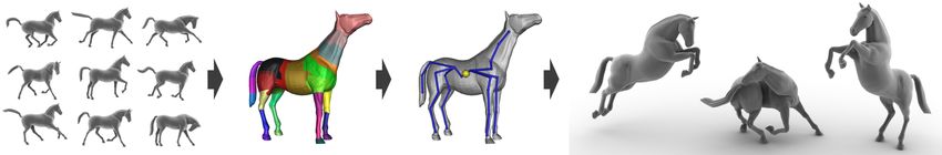
S. Schaefer & C. Yuksel / Example-Based Skeleton Extraction

Figure 1: From a set of example poses we extract clusters representing rigid bones of a skeleton. Next we “skin” the model by
estimating bone weights for each vertex that we then use to determine the connectivity of the skeleton and joint locations. With
this skeleton, we can create new poses outside of the example set including making the horse jump, chase his tail and rear in
the air.

more, since rigid skeletons are supported by most model-              a deformed skeleton associated with them. The authors insert
ing applications, we can manipulate these shapes using pro-           various bones to alleviate traditional problems with skeletal
grams such as Maya without the need for special software or           animation and determine influence sets using a point cluster-
plugins and fit these new deformation models directly into            ing method to solve for vertex weights as well. However both
existing production pipelines.                                        of these skinning techniques assume a skeleton and model
                                                                      are provided for all example poses a priori.
2. Previous Work                                                         Recently, several example-based deformation techniques
Several authors have developed methods for extracting                 have been developed. [JT05] developed a technique for com-
skeletons directly from a static pose of a model using seg-           pressing the storage space needed for an animation or set of
mentation approaches. [KT03] use a fuzzy clustering ap-               poses. The authors accomplish this task by utilizing mean-
proach to develop a hierarchical decomposition of a shape,            shift clustering to robustly determine a set of representative
which a skeleton can then be extracted from. [dATM∗ 04]               transformations associated with the animation. Then the au-
and [TdAM∗ 04] both use voxel descriptions of an object and           thors use non-negative least squares to fit the vertex weights
fit either ellipsoids or superquadrics to estimate a skeleton.        to the transformations and avoid over-fitting in the solution.
Later [KLT05] developed a different segmentation approach             Despite the similarity of this technique to skeletal anima-
based on feature point extraction. [LKA06] also created a             tion, the method is designed to reproduce and compress an
fast decomposition method based on approximate convex                 animation rather than create new deformations. In particular,
decompositions of shape for skeleton extraction as well.              the authors do not build a skeleton to manipulate the shape
                                                                      and utilize affine transformations (uncommon in skeletal de-
   Other methods estimate skeletons from a static pose us-
                                                                      formation) to fit the data better.
ing other data such as feature points [TVD06], various types
of distance functions [LWM∗ 03, MWO03], gaussian curva-                   [SZGP05] also developed an example-based deforma-
ture [MP02] or even probability distributions [FS06]. How-            tion method using deformation gradients and nonlinear min-
ever, these methods are based on a single pose and rarely             imization. Their technique can create very realistic looking
discuss skinning because these weights are difficult to obtain        deformations, but the nonlinear minimization is quite slow
from a static pose and have little to do with how the shape           and limits interactive applications. [DSP06] later improved
actually moves. Furthermore, these techniques may segment             the speed of this method by computing a set of representa-
or extract regions of a shape that are in fact static, like the       tive vertices for use in the minimization, which speeds up
tusks of an elephant, because they are based solely on the            the computation and results in interactive posing.
geometry of the shape.
                                                                         A few researchers have worked on extracting skele-
   The complement to skeletal extraction is skinning. Given
                                                                      tal models from various sources including motion capture
a set of example poses and skeletons associated with each
                                                                      markers [KOF05], 3D range data [AKP∗ 04], and even CT
pose, [WP02] introduce Multi-Weight Enveloping to solve
                                                                      scans of the human hand [KM04]. [AKP∗ 04] extract a skele-
for vertex weights. However, instead of using a single weight
                                                                      ton from 3D range data and clusters rigid components on the
associated with a transformation, the authors allow multiple
                                                                      surface using an an algorithm that iterates between assigning
weights, one for each entry in the transformation matrix. The
                                                                      vertices to clusters through an integer programming prob-
result is a much better fit to the data and smoother deforma-
                                                                      lem and estimation of rigid transformations through an It-
tions though few modeling packages currently support this
                                                                      erated Closest Point algorithm. [KOF05] attempts to extract
technique.
                                                                      a rigid skeleton from the positions of a set of markers from
   [MG03] also take an example-based approach to skin-                motion capture data. Their algorithm determines rigid parts
ning. Again the input is a set of deformed models, each with          by clustering vertices based on the standard deviation of the

                                                                                                        c The Eurographics Association 2007.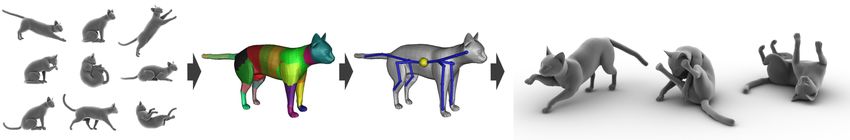
S. Schaefer & C. Yuksel / Example-Based Skeleton Extraction

pair-wise distance between all markers. In our context, these           mesh animations, these disconnected triangles are not prob-
markers correspond to vertices on the surface. While motion             lematic since data reduction is the only goal. However, in
capture data inherently uses a small number of markers, our             skeletal animation, bones are typically associated with com-
surfaces may have 10 to 100 thousand vertices and comput-               pact sets of triangles on the mesh. Therefore, we use a dif-
ing the pair-wise distance between all vertices for clustering          ferent approach to determine the bone transformations.
rigid components is not feasible.
                                                                           Our bone estimation technique is inspired by work in sur-
    [KM04] extract an articulated skeleton from volumet-                face simplification. Algorithms such as QSlim [GH97] use
ric CT data of a hand in various poses as well as provid-               an edge-collapse approach to cluster vertices on the sur-
ing a deformation method based on pose space deforma-                   face. Each vertex has an associated Quadratic Error Func-
tions [LCF00] to capture the subtle skin movement as the                tion whose minimizer determines the location and error of
user manipulates the shape. In contrast to previous tech-               that vertex. The cost of clustering two vertices connected by
niques, the authors do not need to find bone transformations            an edge is then the error of the function that results from
through clustering because the CT data contains the real-               summing the two vertex functions. These vertices are clus-
world bones inside of the hand. In practice, the volumetric,            tered together in a greedy manner until the desired number
skeletal structure is rarely available.                                 of vertices (or polygons) is reached.

Contributions                                                              To find bone transformations, we will find clusters of
                                                                        faces on the surface that transform in a similar manner by
We present a method for estimating the complete set of
                                                                        modifying the standard surface simplification algorithm. The
parameters for skeletal animation including the rigid bone
                                                                        rigid transformations that best describes the motion of each
transformations, skeletal hierarchy, root node, joint locations
                                                                        cluster will then be the transformations associated with each
and vertex weights from a set of example poses. We can then
                                                                        bone in our skeleton.
use this extracted skeleton to create new poses of the char-
acter in a similar fashion to the examples. Since, rigid skele-
tons are supported by most 3D modeling packages, these de-
                                                                        3.1. Rigid Error Functions
formable models fit directly into existing art pipelines. First,
we provide what we call “Rigid Error Functions” that allow              One key piece of the surface simplification algorithm is the
us to efficiently find the best rigid transformation and the            Quadratic Error Function [GH97]. Here we construct its
error of that fit for a set of points using a constant amount           equivalent, the Rigid Error Function for rigid transformation
of space. We then use these error functions to estimate the             simplification. We will assume that we have some set of tri-
transformations of the bones in the example poses with a                angles in parametric form pi (t) from the rest pose and their
fast, face clustering approach. Given these bones, we “skin”            deformed images qki (t) from the kth example pose where t is
the mesh by solving for vertex weights using a constrained              a bivariate parameter. In particular, pi (t) has the form
optimization and bone influence maps. With these weights,
we determine both the connectivity of the skeleton and the                         pi (t) = t1 pi,1 + t2 pi,2 + (1 − t1 − t2 )pi,3
joint locations. Finally, we provide several example models
and drastic, new deformations outside of the example set to             where pi, j is the jth vertex of the triangle pi (t).
demonstrate the robustness of our method.                                  The best rigid transformation R, T that maps the triangles
                                                                        pi (t) to their image qki (t) is given by
3. Bone Estimation                                                                                   Z                        2
                                                                                  Ek (R, T ) = ∑          Rpi (t) + T − qki (t) dt.   (2)
Given a rest pose as well as a set of example poses, our goal                                    i    t
is to estimate a set of bone transformations that govern the
motion of the examples. There are several approaches we                 Now, the best rigid transformation in Equation 2 for the kth
could take to solve this problem. [JT05] present a robust face          example pose is the minimizer of that error function.
clustering method based on mean-shift clustering to extract
these transformations. The advantage of this approach is that                                        min Ek (R, T )
                                                                                                RT R=I,T
the clustering can robustly remove outliers in the data.
   However, the disadvantage is that the method is based                Due to the nonlinear constraint RT R = I, this transformation
on clustering points in a high dimensional space represent-             cannot be found through linear minimization. However, the
ing concatenated rotation matrices. If we are given n exam-             problem contains enough structure that a simple solution still
ples poses, the points lie in a 9n-dimensional space (or 12n-           exists.
dimensional space if translation is used) and nearest neigh-              If we differentiate Equation 2 with respect to T and inte-
bor queries become expensive. Furthermore, the clustering               grate, we find that
does not respect the topology of the mesh and can clus-
ter many disconnected triangles together. For compressing                                            T = q̄k − R p̄

c The Eurographics Association 2007.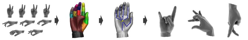
S. Schaefer & C. Yuksel / Example-Based Skeleton Extraction

where p̄, q̄k denotes the area weighted average of the cen-
troids
                                               ∑i ∆i c(pi )
                               p̄     =           ∑i ∆i
                                               ∑i ∆i c(qi )
                                                        k                    (3)
                            q̄k       =           ∑i ∆i
                                                            ,

∆i is the area of the triangle pi (t) and c(pi ) is the centroid
of the triangle pi (t). Substituting this definition into Equa-
tion 2, we find that the error now becomes
                            Z                              2                           Figure 2: Horse skeleton with skin weights shown for differ-
                      ∑        t
                                    R p̂i (t) − q̂ki (t) dt                            ent numbers of bones. From left to right: 29 bones, 19 bones
                        i                                                              and 9 bones.
where  p̂i (t), q̂ki (t) are
                         the triangles with vertices pi, j − p̄ and
 k      k
qi, j − q̄ . Therefore, the best rotation R is given by the polar
decomposition of the matrix                                                            mizer of Ek (R, T ) can likewise be rewritten as
                                    Z
                                                                                                                       2                      2
                                          p̂i (t)q̂ki (t)T dt.                               ∆             2                          2
                        M=                                                   (4)         ∑i 12i 9 |c(pi )| + 9 c(qki ) + ∑3j=1 pi, j + qki, j
                                      t
                                                                                                                                    L

                                                                                                                           2
The polar decomposition has been used many times                                                    −(∑i ∆i ) | p̄|2 + q̄k     − 2M R
in Graphics to find optimal rotations of a set of
points [ACOL00], [MHTG05] and factors a matrix M = RS                                           L
                                                                                       where          denotes component-wise multiplication of
into an orthogonal matrix R and a skew-symmetric matrix S.                             the two matrices followed by summing those products.
Unfortunately, orthogonal does not mean a rotation matrix                              Notice that, in order to compute M, we only need the
as reflections lie in the space of orthogonal matrices. Also,                          scalar ∑i ∆i , the vectors ∑i ∆i c(pi ) and ∑i ∆i c(qki ) as well
the polar decomposition is only defined for matrices of full-

                                                                                       as the matrix ∑i 34 c(qki )c(pi )T + 12     1 3
                                                                                                                                     ∑ j=1 qki, j pTi, j .
rank, meaning that the triangles must span 3-dimensional
space (impossible for a single triangle or planar region of                            Furthermore,       to   compute      the     error      associ-
the surface). Therefore, the polar decomposition can fail to                           ated with the minimizer we need the scalar
                                                                                                                    2                       2
                                                                                          ∆             2                         2
produce the correct solution to this minimization problem.                             ∑i 12i 9 |c(pi )| + 9 c(qki ) + ∑3j=1 pi, j + qki, j      .
   Fortunately, [Hor87] provides an alternative solution                               These sums use a constant amount of space (17 floats) and
based on the eigen-structure of a 4 × 4 symmetric matrix that                          combining two error functions amounts to adding these 17
solves these problems. Given the 3×3 matrix M, we can eas-                             numbers together, which is extremely fast.
ily show that Horn’s 4 × 4 matrix can be found directly from
M [BM92] and is                                                                        3.2. Face Clustering

                Tr(M)               v
                   T        T                                                          Instead of clustering vertices like surface simplification, we
                  v       M + M − Tr(M)I                                               cluster faces. Each non-degenerate face in the rest pose along
where Tr(M) is the trace of the matrix M, I is the 3 × 3                               with its image in an example pose defines a unique, rigid
identity matrix and                                                                    transformation. Therefore, before clustering, we construct a
                                                                                      Rigid Error Function for each face in the rest pose and for
    v = M2,3 − M3,2 M3,1 − M1,3 M1,2 − M2,1 .                                          each example pose. Now each face has n Rigid Error Func-
The unit eigenvector corresponding to the largest positive                             tions associated with it, one for each of the n example poses.
eigenvalue denotes the unit quaternion representing the best                           Next, we connect faces together that share an edge on the
rotation (negative eigenvalues indicate reflections).                                  surface. For each of these adjacent faces, we insert an edge
                                                                                       connecting them into a priority queue whose sort key is the
   Simplification not only requires a method for finding the                           error associated with combining those two faces as defined
best rigid transformation from a set of points, but also ef-                           by their Rigid Error Functions summed over all n examples.
ficient methods for storing and combining these Rigid Error                            Finally we remove edges from the queue with the lowest er-
Functions. We can do so easily by integrating Equation 4 and                           ror and cluster faces together until a specific error tolerance
substituting Equation 3 to form                                                        or a desired number of clusters is reached. Figure 2 shows
                                               !                                       the skeletons created by our algorithm for different numbers
              3 k              1 3 k T
 M = ∑ ∆i                  T
                c(q )c(pi ) +     ∑ qi, j pi, j − q̄k p̄T ∑ ∆i .                       of bones. In general, fewer bones means less work for the
        i     4 i             12 j=1                      i                            user when creating new deformations, but also greater ap-
                                                                                       proximation error.
Assuming that R is the optimal rotation (which can be de-
termined solely from M), the error associated with the mini-                              Notice that this algorithm requires that the mesh is con-

                                                                                                                            c The Eurographics Association 2007.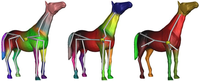
S. Schaefer & C. Yuksel / Example-Based Skeleton Extraction

                                                                        shift clustering though not as robust with respect to outliers.
                                                                        Nevertheless, we have found this technique to be a very
                                                                        good approximation to the rigid movement of the surface.
                                                                        Optionally, we can use a variational technique like Lloyd’s
                                                                        method [CSAD04] with our Rigid Error Functions to at-
                                                                        tempt to improve upon the clusters. In our examples, we
                                                                        have not seen significant improvement with Lloyd’s algo-
                                                                        rithm though it may help with highly deformable objects.

                                                                        4. Skinning: Weight Estimation
                                                                        After clustering, we now skin the rest pose and solve for
Figure 3: The influence of the bone associated with the front
                                                                        weights α j in Equation 1 associated with each vertex to
paw before (left) and after (right) enforcing locality. Without
                                                                        reproduce their positions in the example poses. Several
locality the bone affects not only the paw but the rear feet,
                                                                        example-based skinning methods [WP02, MG03] as well
legs and even the ears all of which will result in undesirable
                                                                        as [JT05] describe methods could be used here. We fol-
deformations when creating new poses.
                                                                        low [JT05] and enforce that the weights produce deforma-
                                                                        tions invariant under rigid transformations (weights for each
                                                                        vertex sum to one) and that each vertex may only be influ-
nected. For surfaces made of disconnected pieces, edges be-             ence by a maximum number of bones (4 for all our exam-
tween faces from separate pieces may need to be created if              ples). Limiting the number of bones allows us to compute
clustering across these disconnected pieces is desired. One             the deformations in an efficient manner using modern GPUs.
automatic method for creating these edges is to connect faces           Furthermore, we require that each α j ≥ 0. While negative
along boundaries with other boundary faces based on prox-               weights may be optimal to reproduce the example poses,
imity information.                                                      they can lead to extremely undesirable deformations when
                                                                        the bones are moved to new poses.
   The implementation of this method is relatively straight-
forward with one caveat. The Rigid Error Functions in Sec-                These constraints lead to a least squares problem for the
tion 3.1 are somewhat expensive to evaluate as they require             weights α j (one for each bone) of the form
n eigenvector computations for the n example poses. Typical                                n
                                                                                                                                 2
surface simplification algorithms perform an edge-collapse,                         min ∑       ∑(α j R j,k pi + Tj,k ) − qi,k
                                                                                     αj
recalculate the error associated with all edges leading to the                            k=1    j
new cluster and reinsert these edges back into the prior-               subject to the constraints
ity queue after each edge-collapse. However, a single edge-
collapse does not just remove one edge, but multiple edges                                           ∑j αj     =     1
(all adjacent clusters connected to both clusters will have one                                         αj     ≥     0 ∀j
edge removed to eliminate redundancy after the collapse).                                  {α j |α j > 0}      ≤     4
Therefore, many of these recalculated edges will never be               where R j,k , T j,k is the minimizer of the Rigid Error Func-
collapsed but removed by neighboring collapses instead.
                                                                        tion for the jth cluster and kth example pose and qi,k is the
   By taking advantage of the inherent monotonic property               position of pi in the kth example pose. This type of least
of the Rigid Error Functions (the collapsed error function              squares problem with equality and inequality constraints can
will have error greater than or equal to the maximum of the             be solved with a general purpose least squares solver with
two children functions), we can improve the performance                 inequality constraints [LH74]. However, our problems are
of this algorithm greatly. After an edge-collapse, we simply            based on skeletal deformation and typically have more struc-
mark the edges connected to this new cluster as dirty instead           ture than a general least squares problem. A simple proce-
of recalculating their errors. When we remove the lowest er-            dure of repeatedly solving the least squares problem with the
ror edge from the priority queue, we check if the edge is               partition of unity constraint and forcing the smallest α j < 0
dirty. If so, we recalculate the error associated with the edge,        to zero until all α j ≥ 0 and 4 or fewer α j ≥ 0 suffices.
mark the edge as clean and reinsert the edge into the pri-
                                                                           The result of this minimization is a set of weights α j for
ority queue. This procedure avoids many costly evaluations
                                                                        each vertex of the surface. These weights still may not pro-
and results in nearly an order of magnitude speed-up in the
                                                                        duce good deformations outside of the example poses be-
algorithm.
                                                                        cause the weights may lack locality, a common property en-
   Figures 1, 4, 6 and 7 show examples of clustering gener-             forced in deformation methods. This lack of locality is the
ated using this method. This process is extremely fast (see             product of bone motions that happen to be correlated in the
Table 1) and is over an order of magnitude faster than mean             example poses but is extremely undesirable when creating

c The Eurographics Association 2007.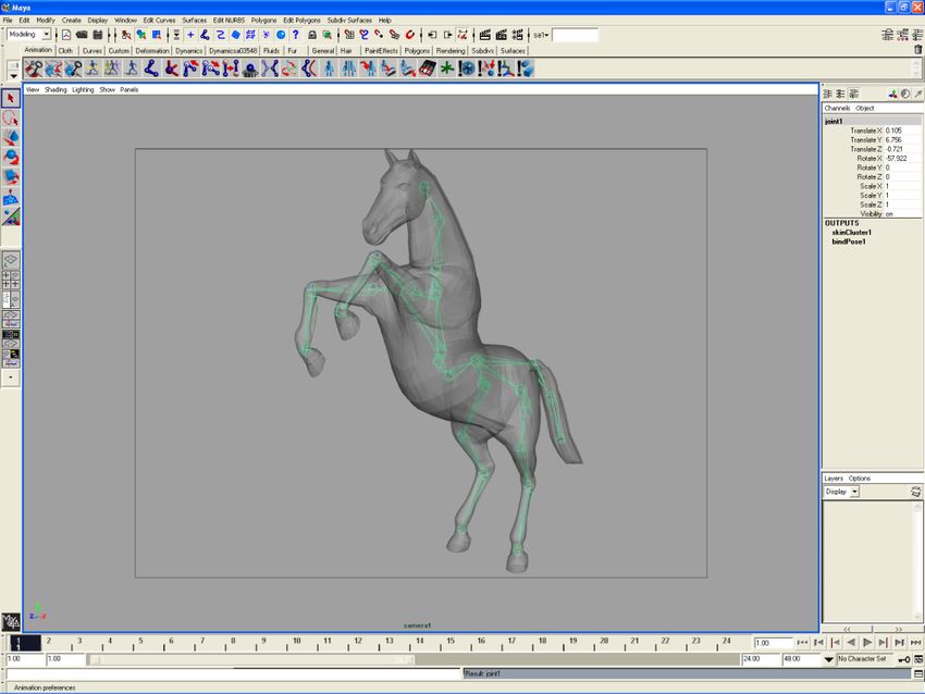
S. Schaefer & C. Yuksel / Example-Based Skeleton Extraction

Figure 4: From left to right: Example poses of a cat, clustering for bone transformations, skeleton found with root shown in
yellow and new poses created using this skeleton.

new poses of the character. Figure 3 (left) shows the influ-          contains the RMS error for each of our examples. As we in-
ence of the bone associated with the front paw of the cat after       crease the number of bones, both measures of error decrease.
minimization. Note how the influence is not connected and             However, increasing the number of bones is not always de-
even influences the back paw and ear of the cat. Even small           sirable and there are more bones that must be manipulated
weights in these disconnected regions can create undesirable          to create new deformations.
deformations as the user manipulates the paw of the cat due
to the lack of locality.
                                                                      5. Skeletal Extraction
   Therefore, we enforce locality by finding an influence
                                                                      So far we have found bone transformations (Section 3) and
map for each bone. For each bone we find the vertex that
                                                                      weights associated with vertices of the mesh (Section 4), but
contains the largest weight and flood outwards until we en-
                                                                      have not created a skeleton to manipulate the shape with.
counter vertices with weight zero with respect to that bone.
                                                                      A skeleton consists of two parts: the connectivity between
We then use these influence maps to restrict the minimiza-
                                                                      bones and the joint locations between pairs of connected
tion to those bones and re-solve for the weights α j . Figure 3
                                                                      bones.
(right) shows the restricted influence map using this tech-
nique. It is possible, though unlikely, that a vertex may not
be covered by any influence map after flooding. In this situ-         5.1. Skeleton Connectivity
ation, we extend the influence maps of the neighboring ver-           Several researchers have taken different approaches to de-
tices to this vertex and repeat until all vertices are covered.       termining skeleton connectivity. [AKP∗ 04] bases the con-
In our examples, our algorithm never had to utilize this step         nectivity of the skeleton on the adjacency information be-
but this case may arise under extreme deformations.                   tween clusters representing rigid components, which works
                                                                      well for tube-like regions where the skeleton connectivity is
                                                                      unambiguous. However, this technique does not produce de-
                                                                      sirable results in regions with more complex adjacency such
                                                                      as the rear of the horse. [KOF05] determine skeleton con-
                                                                      nectivity using a minimum spanning tree approach similar
                                                                      to our method. However, their edge weights are based on a
                                                                      nonlinear measure of the error of placing a joint in between
Figure 5: RMS error for the horse with a variable number              these two bones. We propose a simpler solution based on the
of bones both for the vertex positions and the unit normals           vertex weights from Section 4.
of the polygons. The error for vertex positions is measured               In skeletal animation, vertices of a mesh are typi-
as a percentage of the length of the bounding box diagonal.           cally weighted by multiple, connected bones. These vertex
                                                                      weights actually indicate information about the connectivity
                                                                      of the skeleton. If a vertex is weighted by three bones, then
   Our goal is to develop a set of weights and a skeleton such
                                                                      it is likely that these three bones are connected together in
that a user can create new deformations outside of the exam-
                                                                      some fashion in the skeleton. Therefore, we take advantage
ple set and not just reproduce the example poses. However,
                                                                      of this locality property when determining the connectivity
using these bone transformations and vertex weights, we can
                                                                      between the bones from Section 3.
compare how closely these transformations/weights match
the example poses. Figure 5 shows a plot of the RMS er-                  Our algorithm constructs a weighted edge graph between
ror of the vertex positions as a percentage of the length of          all of the bones of the skeleton and is initially a complete
the diagonal of the bounding box for the rest surface as the          graph with all edge weights set to zero. Next, we iterate
number of bones increases. The RMS of the unit normal is              through all of the vertices in the shape and find their high-
also shown as a function of the number of bones. Table 1 also         est weighted bone. Let max be the index of that bone. Then,

                                                                                                        c The Eurographics Association 2007.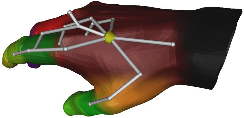
S. Schaefer & C. Yuksel / Example-Based Skeleton Extraction
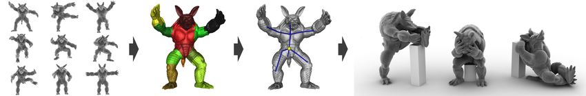
Figure 6: The example poses of this model were created using Mean Value Coordinates, which we successfully convert to a
skeletal deformation model. From left to right: the examples of the armadillo man, clustering for bone transformations, the
extracted skeleton (root shown in yellow) and additional poses created with this skeleton including the stretching, sorrowful
and relaxing armadillo man.
for each j 6= max, we add the weight α j to the edge in the where R1,k , T1,k and R2,k , T2,k are the rigid transformations
connectivity graph between bones j and max. If desired, this associated with the two bones for the kth example pose.
weight α j could be multiplied by the area of the triangles
in the one-ring surrounding this vertex to make the result Many joints like elbows and knees act as hinges and bend
less dependent on the tessellation of the surface, though we along a single axis. This hinge-like action creates an infinite
found no difference in the result for any of our examples. number of minimizers along the axis of rotation. Thus, there
Finally, we extract a maximal spanning tree to determine the may not be a single minimizer to Equation 5, but an entire
final connectivity of the skeleton. Notice that this algorithm subspace. Furthermore, slight noise or variation in the exam-
gives strong emphasis to vertices with nearly equal weights, ple poses may lead to a minimizer in that subspace far away
for instance .5/.5, as an indication of a joint and less empha- from the actual surface.
sis to vertices with more widely spread weights, like .95/.05, Several solutions to this problem have been proposed in-
that may be related to subtle smoothing effects in the exam- volving non-linear minimization [KOF05] and minimizing
ple poses. the distance to the centroid of the boundary [AKP∗ 04]. We
While this algorithm determines the connectivity of the use this idea of minimizing the distance of the joint’s loca-
skeleton, it does not determine the root. The choice of which tion to a point that approximates the joint’s location x̂. The
bone represents the root of the skeleton is somewhat arbi- minimization problem then becomes
trary. Artists will typically choose the pelvis or torso of a min ∑ R1,k (v + x̂) + T1,k − R2,k (v + x̂) + T2,k . (6)
2
human skeleton as the root. For shapes such as snakes, the v
k
choice of the root is less obvious. For our purposes, we de-
termine the root of the skeleton using the center of mass of where v is a vector and we find the solution in the subspace
the shape. The center of mass for a human happens to be which minimizes the magnitude of v. This solution can eas-
near the pelvis or torso, and, given the importance of this ily be found using a pseudoinverse and the final position of
point in physical calculations, there is some physical basis the joint is x = x̂ + v. However, we do not use the centroid
for choosing this point as the root of the skeletal hierarchy. of the boundary for x̂ because the skeleton connectivity al-
Hence, we choose the bone whose corresponding polygons gorithm in Section 5.1 does not require that the connected
from the clustering step have a center of mass closest to that clusters are adjacent on the surface.
of the rest pose as the root of the skeletal hierarchy. Instead, we estimate the joint’s position x̂ using a similar
procedure to Section 5.1. The intuition is that the weights
of the vertices not only indicate information about the con-
5.2. Joint Determination nectivity of the skeleton, but also about the positions of the
joints. For instance a vertex evenly weighted by two bones
Joint determination is a well-studied problem in skeleton ex- (.5/.5) should be very near the joint’s location. Therefore,
traction [AKP∗ 04,KM04,KOF05]. Assume that bones 1 and we find all of the vertices ci ⊆ pi whose maximum weight is
2 are connected. A joint x connecting these two bones has associated with either bone 1 or 2. Let αi, j be the weight for
the property that its location is the same with respect to both ci associated with bone j. We build a weighted average over
bone transformations in all positions. Using this description, all these ci to approximate the joint position as
we define the joint position x as the point that moves the least
with respect to both bones, which leads to the quadratic min- ∑i min(αi,1 , αi,2 )ci
x̂ = .
imization problem ∑i min(αi,1 , αi,2 )
min ∑ R1,k x + T1,k − R2,k x + T2,k This position is refined using the minimization of Equation 6
2
(5)
x
k to create the final placement of that joint.
c The Eurographics Association 2007.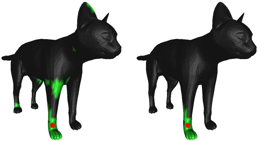
S. Schaefer & C. Yuksel / Example-Based Skeleton Extraction

Figure 7: In the examples (left) the motion of the pinkie and index fingers are nearly identical in all frames. However, our
algorithm successfully extracts separate bones for the skeleton. On the right we show several new examples created with this
skeleton.

6. Results                                                            of the armadillo man’s deformations is known and were pro-
                                                                      duced using 3D mean value coordinates [JSW05]. The defor-
Figures 1, 4, 6 and 7 illustrate our method on several differ-
                                                                      mations created by mean value coordinates are complex, not
ent examples. The number of example poses range from 9
                                                                      local and have no underlying skeletal structure. However, we
(cat and armadillo man) to 46 (the hand example). We de-
                                                                      are still able to extract a skeleton which approximates these
rive the skeletal hierarchy and the joint positions automati-
                                                                      examples.
cally and, in many cases, these skeletons actually resemble
the real-world skeletal structures of these shapes.                      In the example poses for the hand example (Figure 7), the
                                                                      motion of the pinkie and ring fingers are correlated and move
                                                                      in a nearly identical fashion. Transformation clustering ap-
                                                                      proaches [JT05] may not be able to distinguish between the
                                                                      bones of the separate fingers because no topology informa-
                                                                      tion is used. Even clustering points for influence maps using
                                                                      rigidity scores [MG03] can fail in this situation and find cor-
                                                                      relation between the fingers. One solution to this problem is
                                                                      to add more examples poses to demonstrate the disconnected
                                                                      motion of the fingers. However, the topology of the shape
                                                                      provides sufficient information to remove influence between
                                                                      the fingers and our algorithm creates the proper weights for
                                                                      the vertices without the need for further examples.

                                                                         Several of our examples represent animations such as the
                                                                      hand partially closing and opening again. Our method re-
Figure 8: Our system creates a rigid skeleton, which can be           quires very few example poses (as little as one plus a rest
imported directly into standard modeling packages such as             pose) to obtain plausible results. However, we added all
Maya (shown here).                                                    of the animation frames into our optimization to illustrate
                                                                      the running times of the algorithm though fewer frames are
                                                                      needed to create good skeletons.
   Each of these figures also shows several new poses cre-
                                                                         The running times of our algorithm were measured on an
ated with the extracted skeleton and weights. We have also
                                                                      Intel Core 2 6700 PC. Table 1 includes timing results for
implemented a script that loads the rest pose, skeleton and
                                                                      each of the stages of our algorithm on the different exam-
weights directly into Maya for manipulation purposes (see
                                                                      ples. Face clustering is very fast and finishes in a matter of
Figure 8). Since we estimate a standard, rigid skeleton, this
                                                                      a few seconds as opposed to minutes or even close to hours
data fits readily into existing software and requires no special
                                                                      using mean shift clustering. Skinning times encompass both
software beyond standard modeling packages to manipulate
                                                                      the first minimization, finding the influence map and sec-
these shapes.
                                                                      ond minimization. Skeletonization times were trivial in all
   Many of these examples are available freely off the web            examples and almost all under 0.01 seconds. The table also
and the methods used to create these deformations (SSD,               displays the RMS error of the vertex positions as a percent-
FFD, etc...) are unknown. While automatically creating                age of the length of the diagonal for the bounding box of the
skeletons for poses created with skeletal animation is un-            rest shape as well as the RMS error of the unit normal. In all
surprising (though still difficult) our algorithm can be used         cases, our method reproduces the example poses very accu-
to create skeletons for poses that were created using other           rately (less than 1% RMS error) but, more importantly, can
deformation methods. Unlike the other examples, the source            be used to create new poses with our hierarchical skeleton.

                                                                                                         c The Eurographics Association 2007.
S. Schaefer & C. Yuksel / Example-Based Skeleton Extraction
Model Faces Example Bones Face Skinning Skeleton Vertex Normal
Poses Clustering Extraction RMS RMS
Hand 15789 46 19 9.96s 6.46s 0.00s 0.14% 0.09
Horse 16843 23 29 5.53s 11.14s 0.00s 0.29% 0.19
Cat 14410 9 24 2.11s 4.01s 0.00s 0.52% 0.30
Armadillo 30000 9 12 5.21s 2.53s 0.00s 0.75% 0.17
Elephant 84638 23 22 32.29s 32.23s 0.02s 0.34% 0.15
Lion 9996 9 19 1.57s 1.85s 0.00s 0.65% 0.31
Table 1: Running times for various phases of our algorithm with several different models as well as the RMS error for the
position and normal with respect to the example poses. All times are measured in seconds.
Figure 9: Sometimes our algorithm extracts bones whose
motion is really dependent on that of the surrounding bones Figure 10: New poses created from the hand example
as in the case of the knuckle here. spelling out “SGP” in sign language.
7. Future Work
though its motion is solely dependent on the finger bone in
In the future we would like to investigate methods to derive the examples. One solution would be to detect these depen-
parameters for other deformations models for use with flex- dent movements and remove this degree of freedom from the
ible shapes. Skeletal deformation works well for controlling user so that the skin moves automatically with the finger.
shapes that have an underlying biological skeleton or behave
in a nearly rigid manner. However, for flexible shapes such as For symmetric shapes, most users would expect that the
cloth, a skeletal model is not intuitive or appropriate. Our al- skeletons as well as the vertex weights should reflect the ge-
gorithm can be used to derive a skeleton for such shapes, but ometric symmetry of the model. In the armadillo man ex-
interacting with the skeleton may prove difficult. Other de- ample (see Figure 6), the model is symmetric even though
formation methods such as Free-Form Deformations [SP86] the skeleton is clearly not. Currently we do not perform any
may be more appropriate due to their ability to create prov- symmetry detection and our current optimization is based
ably smooth deformations though we must still develop tech- solely on how the object actually moves in the examples.
niques for estimating the parameters for these methods from For the armadillo man, the two halves of the object behave
a set of examples. very differently in the examples and, hence, the skeleton is
not symmetric. A more extreme example might be a person
In some cases, the resulting skeleton is not exactly what a
that has suffered partial paralysis on one side of their body
human would produce. Sometimes the clustering finds rigid
due to a stroke. Even though the geometry of the object is
pieces whose movement is not independent of other bones.
symmetric, we would expect different skeletons based on its
For example, when the figures of the hand bend, the skin on
movement. However, if symmetry is desired, we could ex-
the underside of the palm near the joint or on the knuckle
plore detecting and enforcing such symmetry in the skeleton
moves as well. The motion of the skin in these regions is not
and vertex weights.
the same as the motion of the finger so clustering may de-
cide that this region should be a bone. However, in reality, We would also like to develop a system that allows the
the motion of these parts should be dependent on the only user to input additional information into the training process
the finger bone and not be posable as separate bones. These for our algorithm. For instance, if the user disagrees with
extra bones do not affect the quality of the deformation, but the connectivity of the skeleton that our method develops,
may require more work from the user since there are more they should be able exclude these edges in the connectivity
bones to control. Figure 9 shows an example on the hand graph from the optimization and have the algorithm recreate
where the clustering extracted a bone for the knuckle even a new skeleton that satisfies these constraints. This type of
c The Eurographics Association 2007.S. Schaefer & C. Yuksel / Example-Based Skeleton Extraction
discussion process with the user should lead to an extremely [KT03] K ATZ S., TAL A.: Hierarchical mesh decomposition us-
robust algorithm that requires little user input. ing fuzzy clustering and cuts. ACM Trans. Graph. 22, 3 (2003),
954–961.
Acknowledgements [LCF00] L EWIS J. P., C ORDNER M., F ONG N.: Pose space
We would like to thank Robert Sumner and Jovan Popovic deformation: a unified approach to shape interpolation and
for the models of the horse, cat, elephant and lion and the skeleton-driven deformation. In Proceedings of SIGGRAPH
2000 (2000), pp. 165–172.
Utah 3D Animation Repository for the model of the hand.
[LH74] L AWSON C., H ANSON R.: Solving Least Squares Prob-
lems. Prentice Hall, Englewood Cliffs, NJ, 1974.
References
[LKA06] L IEN J.-M., K EYSER J., A MATO N. M.: Simultaneous
[ACOL00] A LEXA M., C OHEN -O R D., L EVIN D.: As-rigid-as- shape decomposition and skeletonization. In Proceedings of the
possible shape interpolation. In Proceedings of SIGGRAPH 2000 2006 ACM symposium on Solid and physical modeling (2006),
(2000), pp. 157–164. pp. 219–228.
[AKP∗ 04] A NGUELOV D., KOLLER D., PANG H., S RINIVASAN [LSLCO05] L IPMAN Y., S ORKINE O., L EVIN D., C OHEN -O R
P., T HRUN S.: Recovering articulated object models from 3d D.: Linear rotation-invariant coordinates for meshes. ACM
range data. In Proceedings of the Annual Conference on Uncer- Trans. Graph. 24, 3 (2005), 479–487.
tainty in AI (2004).
[LWM∗ 03] L IU P.-C., W U F.-C., M A W.-C., L IANG R.-H.,
[BM92] B ESL P. J., M C K AY N. D.: A method for registration of
O UHYOUNG M.: Automatic animation skeleton construction us-
3-d shapes. IEEE Trans. Pattern Anal. Mach. Intell. 14, 2 (1992),
ing repulsive force field. In Proceedings of Pacific Graphics 2003
239–256.
(2003), p. 409.
[BPGK06] B OTSCH M., PAULY M., G ROSS M., KOBBELT L.:
[MG03] M OHR A., G LEICHER M.: Building efficient, accurate
Primo: Coupled prisms for intuitive surface modeling. In Euro-
character skins from examples. ACM Trans. Graph. 22, 3 (2003),
graphics Symposium on Geometry Processing (2006), pp. 11–20.
562–568.
[CSAD04] C OHEN -S TEINER D., A LLIEZ P., D ESBRUN M.:
Variational shape approximation. In SIGGRAPH ’04: ACM SIG- [MHTG05] M ÜLLER M., H EIDELBERGER B., T ESCHNER M.,
GRAPH 2004 Papers (2004), pp. 905–914. G ROSS M.: Meshless deformations based on shape matching.
ACM Trans. Graph. 24, 3 (2005), 471–478.
[dATM∗ 04] DE AGUIAR E., T HEOBALT C., M AGNOR M.,
T HEISEL H., S EIDEL H.-P.: m3 : Marker-free model reconstruc- [MP02] M ORTARA M., PATANÉ G.: Affine-invariant skeleton of
tion and motion tracking from 3d voxel data. In Proceedings of 3d shapes. In SMI ’02: Proceedings of Shape Modeling Interna-
Pacific Graphics 2004 (2004), pp. 101–110. tional 2002 (SMI’02) (2002), p. 245.
[DSP06] D ER K. G., S UMNER R. W., P OPOVI Ć J.: Inverse kine- [MWO03] M A W.-C., W U F.-C., O UHYOUNG M.: Skeleton ex-
matics for reduced deformable models. In SIGGRAPH ’06: ACM traction of 3d objects with radial basis functions. In SMI ’03: Pro-
SIGGRAPH 2006 Papers (2006), pp. 1174–1179. ceedings of Shape Modeling International 2003 (2003), p. 207.
[FS06] F ELDMAN J., S INGH M.: Bayesian estimation of the [SP86] S EDERBERG T. W., PARRY S. R.: Free-form deformation
shape skeleton. J. Vis. 6, 6 (6 2006), 23–23. of solid geometric models. In Proceedings of SIGGRAPH 1986
(1986), pp. 151–160.
[GH97] G ARLAND M., H ECKBERT P.: Surface simplification us-
ing quadric error metrics. In Proceedings of SIGGRAPH 1997 [SZGP05] S UMNER R. W., Z WICKER M., G OTSMAN C.,
(1997), pp. 209–216. P OPOVI Ć J.: Mesh-based inverse kinematics. In SIGGRAPH
’05: ACM SIGGRAPH 2005 Papers (2005), pp. 488–495.
[Hor87] H ORN B.: Closed-form solution of absolute orientation
using unit quaternions. Journal of the Optical Society of America [TdAM∗ 04] T HEOBALT C., DE AGUIAR E., M AGNOR M. A.,
A 4, 4 (April 1987), 629–642. T HEISEL H., S EIDEL H.-P.: Marker-free kinematic skeleton
[JSW05] J U T., S CHAEFER S., WARREN J.: Mean value coor- estimation from sequences of volume data. In VRST ’04: Pro-
dinates for closed triangular meshes. In SIGGRAPH ’05: ACM ceedings of the ACM symposium on Virtual reality software and
SIGGRAPH 2005 Papers (2005), pp. 561–566. technology (2004), pp. 57–64.
[JT05] JAMES D. L., T WIGG C. D.: Skinning mesh animations. [TVD06] T IERNY J., VANDEBORRE J.-P., DAOUDI M.: 3d mesh
ACM Transactions on Graphics (SIGGRAPH 2005) 24, 3 (Aug. skeleton extraction using topological and geometrical analyses.
2005). In Proceedings of Pacific Conference 2006 (Taipei, Taiwan, Oc-
tober 11-13 2006).
[KLT05] K ATZ S., L EIFMAN G., TAL A.: Mesh segmentation
using feature point and core extraction. The Visual Computer 21, [WP02] WANG X. C., P HILLIPS C.: Multi-weight enveloping:
8-10 (2005), 649–658. least-squares approximation techniques for skin animation. In
Proceedings of the Symposium on Computer Animation 2002
[KM04] K URIHARA T., M IYATA N.: Modeling deformable hu-
(2002), pp. 129–138.
man hands from medical images. In SCA ’04: Proceedings of the
symposium on Computer animation (2004), pp. 355–363. [YZX∗ 04] Y U Y., Z HOU K., X U D., S HI X., BAO H., G UO B.,
S HUM H.-Y.: Mesh editing with poisson-based gradient field
[KOF05] K IRK A. G., O’B RIEN J. F., F ORSYTH D. A.: Skeletal
manipulation. In SIGGRAPH ’04: ACM SIGGRAPH 2004 Pa-
parameter estimation from optical motion capture data. In CVPR
pers (2004), pp. 644–651.
2005 (2005), pp. 782–788.
c The Eurographics Association 2007.You can also read