Slurm: fluid particle-in-cell code for plasma modeling
←
→
Page content transcription
If your browser does not render page correctly, please read the page content below
Slurm: fluid particle-in-cell code for plasma modeling
                                                             V. Olshevskya,b,∗, F. Bacchinia , S. Poedtsa , G. Lapentaa
arXiv:1802.08838v2 [physics.comp-ph] 24 Jun 2018

                                                    a
                                                     Centre for mathematical Plasma Astrophysics (CmPA), KU Leuven. Celestijnenlaan
                                                                        200B, bus 2400, B-3001 Leuven, Belgium
                                                   b
                                                     Main Astronomical Observatory, 27 Akademika Zabolotnoho St. 03143, Kyiv, Ukraine

                                                   Abstract
                                                   With the approach of exascale computing era, particle-based models are be-
                                                   coming the focus of research due to their excellent scalability. We present a
                                                   new code, Slurm, which implements the classic particle-in-cell algorithm for
                                                   modeling magnetized fluids and plasmas. It features particle volume evolu-
                                                   tion which damps the numerical finite grid instability, and allows modeling of
                                                   key physical instabilities such as Kelvin-Helmholtz and Rayleigh-Taylor. The
                                                   magnetic field in Slurm is handled via the electromagnetic vector potential
                                                   carried by particles. Numerical diffusion of the magnetic flux is extremely
                                                   low, and the solenoidality of the magnetic field is preserved to machine pre-
                                                   cision. A double-linked list is used to carry particles, thus implementation of
                                                   open boundary conditions is simple and efficient. The code is written in C++
                                                   with OpenMP multi-threading, and has no external dependencies except for
                                                   Boost. It is easy to install and use on multi-core desktop computers as well
                                                   as on large shared-memory machines. Slurm is an ideal tool for its primary
                                                   goal, modeling of space weather events in the heliosphere. This article walks
                                                   the reader through the physical model, the algorithm, and all important de-
                                                   tails of implementation. Ideally, after finishing this paper, the reader should
                                                   be able to either use Slurm for solving the desired problem, or create a new
                                                   fluid PIC code.
                                                   Keywords: particle-in-cell, magnetohydrodynamics, plasma simulations,
                                                   computational fluid dynamics

                                                        ∗
                                                       Corresponding author
                                                       Email addresses: vyacheslav.olshevsky@kuleuven.be (V. Olshevsky),
                                                   fabio.bacchini@kuleuven.be (F. Bacchini), stefaan.poedts@kuleuven.be
                                                   (S. Poedts), giovanni.lapenta@kuleuven.be (G. Lapenta)

                                                   Preprint submitted to Computer Physics Communications                June 26, 2018
1. Motivation
    Particle-in-cell (PIC) method was first proposed by Harlow (1964) for
modeling compressed fluids. PIC combines particles which follow material
motion and carry conserved quantities such as mass and momentum, with a
grid on which the equations of motion are solved. Computational particles
in PIC could be considered as a moving refined grid, hence the method is
useful for modeling highly distorted flows and interface flows. Early imple-
mentations were cumbersome (especially in treating boundary conditions),
memory-hungry, and unable to treat certain physical problems such as, e.g.,
stagnating flows, which made the method obsolete. However, in the last two
decades the method got its second wind thanks to the Cloud-in-Cell (CIC)
algorithm (Langdon and Birdsall, 1970) for kinetic modeling of plasmas, and
the Material Point Method (MPM) applied in solid mechanics (Sulsky et al.,
1995). It is common nowadays to treat PIC solely as a method for kinetic
plasma modeling, therefore narrowing its scope only to CIC (Brackbill, 2005).
Both MPM and CIC delivered impressive new results and are further devel-
oping; we refer the reader to the reviews of the applications of CIC in space
plasma modeling (Lapenta, 2012); MPM in geophysics (Sulsky et al., 2007;
Fatemizadeh and Moormann, 2015), engineering (York et al., 2000), and 3D
graphics (Stomakhin et al., 2013).
    Motivated by the above success we proposed a new PIC algorithm for
magnetized fluids (Bacchini et al., 2017) which clarified and simplified many
aspects of the original FLIP-MHD algorithm by Brackbill (1991). This article
discusses the realization of our algorithm, Slurm, implemented in C++ with
OpenMP multi-threading. We will walk you through all steps of the typical
computational cycle of Slurm, its initialization, and main solver loop, ex-
plaining, where appropriate, data structures, architecture and physical mod-
els used in the code.

2. Physical model
2.1. MHD equations
    Slurm is designed (but not limited) to numerically advance in time a
discretized set of conventional MHD equations in Lagrangian formulation

                                     2
which describe the dynamics of plasmas or magnetized fluids
        dρ       ∂ul
            = −ρ     ,                                                                 (1)
        dt       ∂xl

        duj      ∂p              ∂           1 2
      ρ      =−        + ρgj +       Bi Bj − B δij +
         dt      ∂xj            ∂xi          2

                              ∂       ∂uj ∂uj              2     ∂ul
                                   µ       +        + µv − µ         δij ,             (2)
                             ∂xi      ∂xi    ∂xi           3     ∂xl
                                                   2         2
        de       ∂ul         ∂uj ∂uj       2 ∂ul            ∂ul
      ρ = −p           +µ         +      −       δij + µv          + ηJ 2 ,            (3)
         dt      ∂xl         ∂xi     ∂xi   3 ∂xl            ∂xl
where summation is implied over the repeating indices i, j, l, which denote
vector components; d/dt = ∂/∂t + uj ∂/∂xj is the convective derivative. The
plasma is described by density ρ, velocity u, pressure p, internal energy per
unit mass e, and magnetic field B; g represents external forces (gravity);
µ = νρ is the dynamic shear viscosity and µv = νv ρ is the dynamic bulk
viscosity1 ; η is the resistivity, and J = ∇ × B is electric current; δij is the
Kronecker delta.
    In most cases reported in this paper, the adiabatic equation of state is
assumed
                                        1 p
                                    e=        ,                              (4)
                                        ργ −1
where γ is the predefined gas constant.

2.2. Magnetic field equation
    To close the above system of MHD equations, a condition must be im-
posed on the evolution of B. As a proxy for magnetic field, Slurm uses
electromagnetic potentials A and φ, where

                                      B = ∇ × A.                                       (5)

Using vector potential as a proxy for magnetic field, on a staggered grid (Yee
lattice), the ∇ · B = 0 condition is satisfied to machine precision (Bacchini
et al., 2017). The staggered grid also makes our method second-order ac-
curate in space. In Slurm, the magnetic field is specified on the grid’s cell
centers, and electromagnetic vector potential is given on cell vertices (nodes).

  1
      the notation and terminology follows the excellent book by Kundu et al. (2012)

                                            3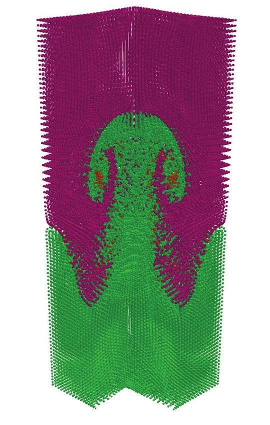
The evolution of A is governed by the equation
                    dA
                       = u × B + (u · ∇) A − ∇φ − ηJ,                      (6)
                    dt
where φ can be chosen freely to satisfy a certain gauge condition. Although it
has no effect on the solenoidality of the magnetic field, appropriate measures
have to be taken to preserve the gauge condition throughout the simulation.
Tricco and Price (2012); Tricco et al. (2016) have introduced the constrained
hyperbolic divergence cleaning of ∇ · B in smoothed particle hydrodynamics,
which was used later by Stasyszyn and Elstner (2015) to clean the divergence
of A. According to this strategy, the scalar potential φ is evolved as
                           dφ                σch
                              = −c2h ∇ · A −     φ,                        (7)
                           dt                 h
where ch is the fast MHD wave speed, h is the smoothing length (particle
size), and σ ≈ 1 is a constant. This way, the Coulomb gauge ∇ · A = 0 or
any other initial gauge could be preserved throughout the simulation.
    Interestingly, in two dimensions
                                    ∂Az
                                Bx =     ,                                 (8)
                                     ∂y
                                     ∂Az
                              By = −      ,                                (9)
                                      ∂x
and by definition
                                  dAz
                                      = 0,                              (10)
                                   dt
hence Az defined on a moving grid (particles), does not change over time
(Bacchini et al., 2017). Therefore in 2D (with no out-of-plane B field) the
gauge condition is preserved to roundoff, and no divergence cleaning is nec-
essary.

2.3. Artificial viscosity
    The PIC method has very low numerical dissipation, and in many prob-
lems related to shock handling a numerical bulk viscosity µυ is useful to
stabilize the solution. Among many possible options we had tested, we ob-
tained satisfactory results with the Kuropatenko’s form of artificial viscosity

                                       4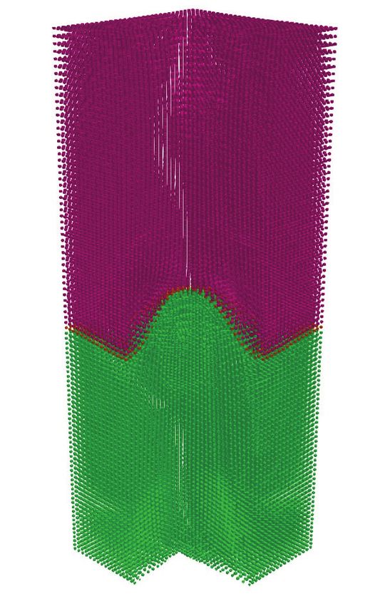
(Kuropatenko, 1966; Chandrasekhar, 1961). This viscosity is non-zero only
in grid cells for which ∇ · u > 0. As given by Caramana et al. (1998),
s
2
γ+1 γ+1
µυ = ρ c2 |∆u| + c22 (∆u)2 + c21 c2s |∆u| , (11)
4 4
wherep|∆u| = |∆ux + ∆uy + ∆uz | is the velocity jump across the grid cell,
cs = γp/ρ is the adiabatic sound speed, c1 and c2 are constants close to 1.
3. Main classes and data structures
Traditional implementations of PIC (or, rather, CIC) algorithms use con-
ventional domain decomposition for parallelizing the computation which, ob-
viously, can lead to strong processor load imbalance. Different strategies
were proposed to overcome it, such as particle splitting/merging (Beck et al.,
2016) or grid refinement and temporal sub-stepping (Innocenti et al., 2015).
Particle methods, instead, provide excellent opportunity for task or event
based parallel approach. The latter has been discussed by, e.g., Karimabadi
et al. (2005), but no productive implementation has been reported yet, to
our knowledge.
Slurm embraces a task based approach in which all particle operations are
split between a user-defined number of OpenMP threads. Distributing tasks,
not computational sub-domains, is advantageous in problems with strong
density imbalances. Particles and computational grid exchange information
several times during each computational cycle, but otherwise grid operations
and particle operations are independent. Therefore two main classes, Grid
and ParticleManager, were chosen to manage grid elements (cells and nodes)
and particles, respectively.
3.1. Basic players: cells, nodes, and particles.
We use a staggered grid, therefore three types of basic entities are repre-
sented by the GridCell, GridNode, and Particle classes, which share some
common properties as illustrated in Fig. 1. Particles carry the following
physical quantities: volume V , mass m, momentum mu, internal energy
= em, and electromagnetic potentials A and φ (the latter is solely used
to preserve the gauge of A). Each grid element is assigned a mass m and a
volume V , hence the density is computed (upon interpolation from particles)
5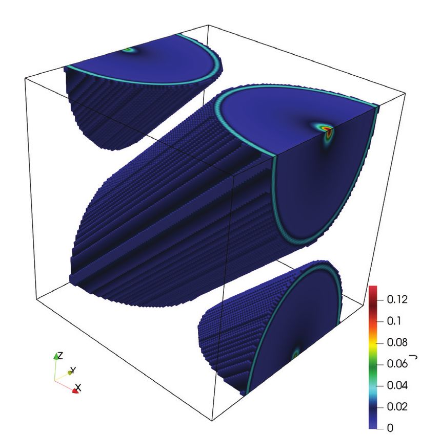
GridPoint
                                                x, y, z

                                            MaterialPoint
                                              m, V, ρ

                                   GridElement          Particle
                                     i, j, k, …        mu, A, ε, ϕ

                            GridCell          GridNode
                             e, B, ϕ             u, A

Figure 1: Inheritance diagram for the basic entities in Slurm: points, grid elements and
particles. Letters in each box indicate basic physical quantities carried by the correspond-
ing item.

as ρ = m/V , for both nodes and cells. Grid nodes keep the fluid velocity
u and the vector potential A, while grid cells keep the internal energy den-
sity e, the magnetic field B and the scalar potential φ. In addition, all grid
elements carry connectivity information as explained below.

3.2. Grid
    The Grid object is initialized by the solver first. Slurm supports rectilinear
grids with nxc × nyc × nzc cells in each dimension, and nxn × nyn × nzn nodes
in each dimension (nx,y,z n = nx,y,z c + 1). At each boundary, there is one
layer of ghost cells, one layer of ghost nodes. Each cell and each node stores
information about its role (‘general’, ‘boundary’, or ‘ghost’) and pointers
to its neighbors. Besides geometrical neighbors, logical neighbors are also
computed.
    Logical neighbors denote the grid elements which must be used for inter-
polating to/from this grid element. For instance, a ‘logical neighbor node’ of
a boundary cell on a periodic boundary is the node on the opposite boundary.
The number of particles is much larger than the number of grid elements,

                                             6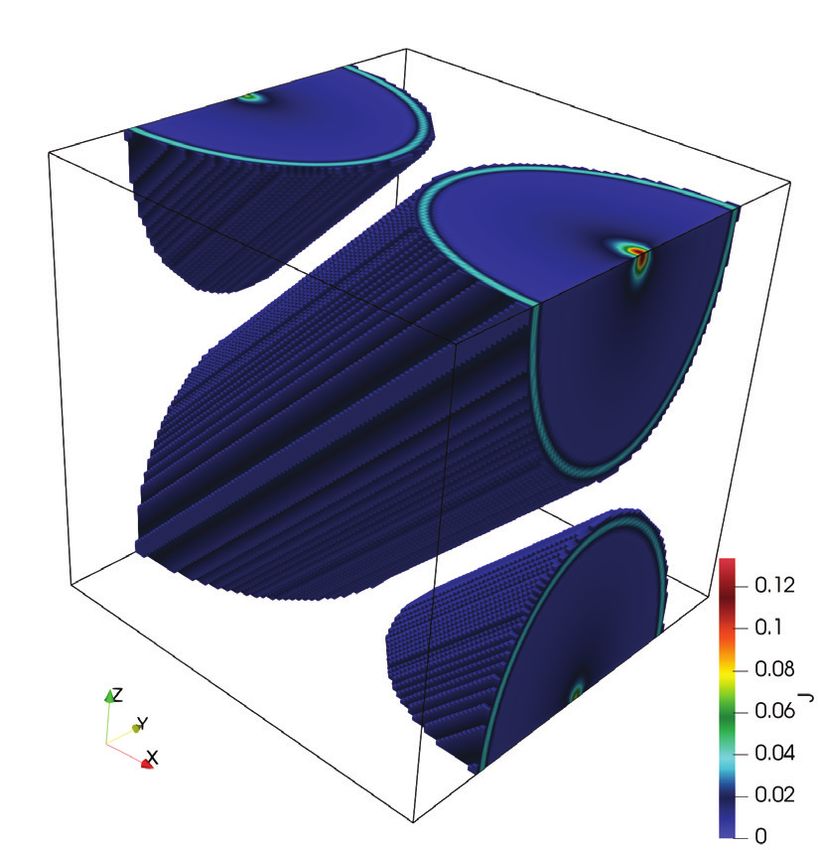
hence connectivity information doesn’t lead to excessive memory use. How-
ever, it saves a substantial amount of resources and provides capabilities for
implementing irregular grids.

3.3. Particle Manager
    . Class ParticleManager stores a double-linked list of Particle objects,
which makes adding and removing particles rather efficient and trivial to
implement. The list could easily be processed in parallel using OpenMP
directives, e.g.,
  #pragma omp parallel
  {
    int thread_num = omp_get_thread_num();

       // Make sure particles were divided between threads according
      to the current number of threads
       if (omp_get_num_threads() != IteratorsNumberOfThreads)
       {
         if (thread_num == 0)
           IteratorsNumberOfThreads = omp_get_num_threads();

          #pragma omp barrier
          computeOMPThreadRange();
      }

       // Process particles which belong to this thread.
       for(ParticleIterator pi = IteratorsBegin[thread_num]; pi !=
      IteratorsEnd[thread_num]; ++pi)
       {
         // Do something
       }
  }

where IteratorsNumberOfThreads is the number of threads for which the par-
ticle ranges IteratorsBegin and IteratorsEnd were computed. All expensive
procedures: interpolation from particles to grid, interpolation from grid to
particles, and particle push, are handled by the ParticleManager object, and
are parallelized in the above manner.
    Strong scaling tests performed on 36-core Intel Xeon processor E5-2600 v4
(Broadwell) have shown that parallel performance improves with the number

                                      7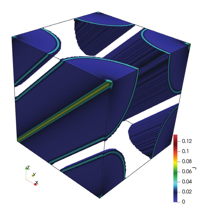
Figure 2: Strong scaling on Intel Xeon E5-2600 v4 (Broadwell). The black line denotes
ideal scaling; each color line corresponds to the number of particles per cell: from 27 to
216. The more particles per cell, the better the scaling is.

of particles per cell (Figure 2). To compute the parallel speedup, we ran
simulations on the same 323 grid, increasing the number of threads from 1
to 36. The parallel speedup equals to the ratio of the average time of one
computational cycle on one thread to the time on multiple threads s(N ) =
hT (1)i / hT (N )i. On 36 threads the code executes 18 times faster than on a
single thread, i.e., parallel efficiency reaches 50%. Note, the code has neither
been optimized, nor tuned for performance. We used GNU C++ compiler
6.1 with the following options: -std=c++11 -O3 -fopenmp -lpthread.

4. Main solver loop
    The main solver loop of an explicit PIC algorithm consists of four steps:
(1) interpolation particles→grid, (2) grid advancement, (3) interpolation
grid→particles, and (4) particle mover, as illustrated in Figure 3. In a typ-
ical PIC simulation the number of computational particles far exceeds the
number of grid cells, and traversing all particles is the most time-consuming
operation in the cycle. In Slurm, particles are only traversed twice per cycle:
first time in step (1) to interpolate to the grid. The second loop invokes both
grid→particle interpolation and particle push, therefore steps (3) and (4) are
combined. In the same loop particles are confronted against the boundary

                                            8
Interpolate to grid
nodes: mu, m, V, A
cells: e, m, V, ϕ
Advance grid
Advance particles
nodes: u, A
r, u, ε , V, A , ϕ
cells: e, grad(u), ϕ
Interpolate to particles
nodes: u, Δu, ΔA
cells: Δe, grad(u), Δϕ
Figure 3: Four-step explicit particle-in-cell algorithm implemented by Slurm.
conditions, and are marked for deletion if needed.
4.1. Step 1. Interpolation from particles to grid.
Projection of data from particles to grid begins with setting the corre-
sponding quantities (m, V , e, φ for cells and m, V , u, A for nodes) to zero.
Interpolation is implemented in the ParticleManager class in one loop over
all particles. It fetches the required information from each particle and adds
the corresponding contribution to the surrounding grid nodes and grid cells.
When all particles have been processed, the accumulated values of the phys-
ical quantities on each grid element are normalized to the total interpolated
weight at that grid element.
Information from each particle (, m, V , V φ) is projected onto 27 cells:
9the cell that encloses this particle, and 26 cells that share a face or a vertice
with it. Interpolation weights are given by the second order b-spline
(
1 2
2
x − 23 |x| + 98 12 ≤ |x| < 32
wc,x = , (12)
−x2 + 43 0 ≤ |x| < 12
where x = (xc − xp ) /∆x is the difference between the cell center coordinate
xc and the particle’s coordinate xp normalized to the cell’s extent ∆x. The
total weight is the product of the three weights in each dimension
wc = wc,x · wc,y · wc,z (13)
Conserved quantities to be projected on the nodes include um, m, V .
These are interpolated onto 8 vertices (nodes) of the cell which encloses this
particle. To compute interpolation weights, the conventional first order b-
spline is used as described in Bacchini et al. (2017)
wn = (1 − |xn − xp |) · (1 − |yn − yp |) · (1 − |zn − zp |) , (14)
where xn , yn , zn are the coordinates of this vertex (node). A different pro-
cedure used to interpolate A from particles to grid.
Electromagnetic vector potential is not an additive conserved quantity,
but rather a smooth vector function of three coordinates. We interpolate
A to each grid node from an arbitrary hexahedron formed by the node’s
closest particles. Each grid node keeps information about the eight closest
particles, hence the interpolation is realized in the Grid class. It is called
when all conserved quantities have been projected. Interpolation from irreg-
ular grids is quite straightforward in 2D2 , but in three dimensions it is more
sophisticated, and requires the iterative solution of a nonlinear system. For
the sake of completeness, we provide the detailed description of the interpo-
lation procedure adopted from NASA’s b4wind User’s Guide3 in Appendix
A. Note, the same interpolation approach may be used for projecting the
scalar potential φ on the cells, however none of our tests indicated that this
is beneficial.
2
https://www.particleincell.com/2012/quad-interpolation
3
https://www.grc.nasa.gov/WWW/winddocs/utilities/b4wind guide/trilinear.html
104.2. Step 2. Advance the grid
4.2.1. Boundary conditions
Boundary conditions should applied to all quantities interpolated from
particles, and to all derived quantities such as B and J. All ghost and bound-
ary grid cells and nodes carry the references to the applicable BoundaryCondition
objects. They implement methods which modify the given cell or node
quantities according to the specific rule. For instance, in reflective boundary
// class BoundaryConditionReflective : public BoundaryCondition
void BoundaryConditionReflective::imposeOnNode(GridNode * n,
SlurmDouble t)
{
for (SlurmInt i = 0; i < 3; i++)
if (i == normal)
n->set_u(normal, 0);
else
n->set_u(i, 2 * n->get_u(i));
n->set_m(2 * n->get_m());
}
4.2.2. Directional derivatives
To evolve the equations of MHD in time, and to compute certain derived
quantities such as B, J, etc., the gradients or directional derivatives of the
discretized quantities should be computed. In Slurm, a directional derivative
of a node quantity q in the direction x is cell-centered. It is computed as the
average over the four corresponding edges of that cell. Using three indices i,
j, k, corresponding to x, y, z coordinate dimensions, we designated the node-
centered value as qijk , where each index is either 0 for the ‘left’ (bottom,
front) or 1 for the ‘right’ (top, back) corner of the given cell. Then the
discrete directional derivatives are equal to
∂q q100 − q000 + q110 − q010 + q101 − q001 + q111 − q011
= , (15)
∂x 4∆x
∂q q010 − q000 + q110 − q100 + q011 − q001 + q111 − q101
= , (16)
∂y 4∆y
∂q q001 − q000 + q101 − q100 + q011 − q010 + q111 − q110
= , (17)
∂z 4∆z
11where ∆x, ∆y, and ∆z are the cell’s extents in the corresponding dimension.
The gradients of cell-centered quantities are node-centered. They are com-
puted in exactly the same way, except that ∆x, ∆y, and ∆z should represent
the distances between the corresponding neighbor cell centers. This way, the
second derivative of a node quantity is node-centered, and the second deriva-
tive of a cell quantity is cell-centered.
4.2.3. Solution of MHD equations
A semi-implicit scheme is used to march the MHD equations on the grid
in time. First, from the cell-centered properties at the previous time step n,
the new velocity is computed on each node.
un+1 = un + ∆tQn , (18)
where Qn is the right-hand side of the discretized momentum equation 2
computed with the ‘old’ grid values. Other grid properties are advanced
using the new velocity according to discretized equations 1, 3, 6, 7, after the
boundary conditions are imposed on un+1
q n+1 = q n + ∆tQ un+1 , ρn , pn , An , φn ,
(19)
where q is one of ρ, e, A, or φ, and Q is the right-hand side of the corre-
sponding MHD equation. Note, boundary conditions need to be taken care
of before interpolating the updated information to the particles.
The numerical scheme described above is a special case of the implicit
scheme analyzed by Brackbill and Ruppel (1986). It is stable when the
Courant condition is met, and offers better accuracy than a simple foward
Euler method.
4.3. Steps 3 and 4. Interpolate on, and push the particles
The weights used to interpolate from grid to particles are the same as
those used for particles to grid projection (Section 4.1). From grid cells
to particles we interpolate the change of internal energy ∆ = n+1 − n ,
the cell-centered velocity gradient ∇un+1 , and the change of scalar potential
∆φ = φn+1 − φn . From grid nodes, the following quantities are interpolated:
un+1 , ∆u = un+1 − un , and ∆A = An+1 − An .
12Physical quantities carried by the p − th particle are updated as
n+1
p = np + mp ∆e, (20)
un+1
p = unp + ∆u, (21)
An+1
p = Anp + ∆A, (22)
φn+1
p = φnp + ∆φ. (23)
The velocity gradient is used to advance the particle’s volume according to
either the strategy described by Bacchini et al. (2017), or in a simpler way:
Vpn+1 = Vpn 1 + ∆t Tr ∇un+1 ,
(24)
where
Tr ∇un+1 ≡ ∇ · un+1 = ∇un+1 n+1 n+1
11 + ∇u22 + ∇u33 (25)
is the trace of the interpolated velocity gradient tensor. Note that particle
quantities are updated using the interpolated changes in the grid quanti-
ties (∆q), which ensures very low numerical diffusivity of the method. The
interpolated velocity un+1 is used only to advance the particle’s position
rn+1 = rn + un+1 ∆t. (26)
Once the new position is found, it is checked against boundary conditions.
If necessary, the particle is either reflected from the wall, flipped around the
periodic boundary, or marked for deletion if it crosses an open boundary.
When all particles have been updated, the list of particles is walked
through one more time, and all particles marked for deletion are removed.
Finally, if necessary, new particles are injected and the pre-computed particle
ranges for each thread are updated.
5. Examples
Most testcases considered in this section could be directly compared with
an excellent paper on Athena code validation by Stone et al. (2008). Where
appropriate, we provide references to the corresponding figures in this paper.
131.61e1 8
1.4 a 7 b
1.2 6
1.0 5
0.8 4
0.6 3
0.4 2
0.2 1
0.0 0
0.20.0 0.2 0.4 0.6 0.8 1.0 1
0.0 0.2 0.4 0.6 0.8 1.0
Figure 4: Simulations of the two interacting blast waves at two resolutions, with 2400 cells
(solid line), and with 200 cells (crosses), at t = 0.038.
5.1. Two interacting blast waves
A simple one-dimensional 1D shock tube proposed by Woodward and
Colella (1984) is widely used to study the shock-capturing and stability
properties of the codes. In this problem, the initial state posesses a uni-
form density ρ = 1, specific heats ratio γ = 1.4, zero velocity, and three
different pressures. In the leftmost tenth of the domain p = 1000, in the
rightmost tenth p = 100, and in between p = 0.01. The shock tube evolves
quickly and produces multiple shock waves at high Mach numbers which are
reflected from the walls and interact with each other. This test is very hard
to handle for Eulerian codes, however Slurm deals with it rather easy. Step-
by-step description of the complex evolution could be found in Woodward
and Colella (1984), we only present the final result at time t = 0.038.
We performed two runs, with 2400 and 200 cells; both with 40 particle/-
cell, and the same ∆t = 4 · 10−6 . The CFL condition computed p on the fine
grid using the largest initial value of the sound speed cs = γp/ρ = 37.4
suggests ∆t < 1.1 · 10−5 . The density and velocity profiles at t = 0.038 in
both simulations are shown in Figure 4. These plots can be compared to the
reference solutions in Figure 2h of the original paper (Woodward and Colella,
1984). Even at low grid resolution (200 cells), the contact discontinuity at
x = 0.6 (Fig. 4b) is very sharp. However, even at high resolution there is
an artificial spike at density discontinuity at x = 0.8. This spike neither
grows, nor is a source of fictious oscillations, even when the simulation is run
141.0 1.0 b
FR SM a
0.8 0.5
0.6 C 0.0
0.4
0.2 SS FR 0.5
0.0 1.0
0.0 0.2 0.4 0.6 0.8 1.0 0.0 0.2 0.4 0.6 0.8 1.0
0.8 0.0
0.6 c d
0.4 0.5
0.2 1.0
0.0 1.5
0.2
0.40.0 2.0
0.2 0.4 0.6 0.8 1.0 0.0 0.2 0.4 0.6 0.8 1.0
Figure 5: Simulations of Brio & Wu shock tube at two resolutions, with 3200 cells (solid
line), and with 400 cells (crosses), at t = 0.1.
further. More sophisticated forms of hyperviscosity might be needed to get
rid of it in our simple explicit first-order numerical scheme.
5.2. Brio & Wu shock tube
Brio and Wu (1988) proposed an extension of the Sod shock tube to MHD.
There are two initial states in the initial domain with Lx = 1: the left state
has ρ = 1, p = 1, and By = 1; the right state has ρ = 0.125, p = 0.1, and
By = −1. In the whole domain, Bx = 0.75, γ = 2, and all other quantities
are zero. In terms of vector potential, the initial field is given by
(
−x 0 ≤ x < 0.5
Az = . (27)
x − 1 0.5 ≤ x ≤ 1
At each computational cycle, when B is computed on grid cells from the
interpolated A according to Eq. 5, Bx = 0.75 is added in each cell.
The aim of this test is to check how well the code distinguishes and
handles different MHD shocks. We present here the results of two runs: with
15Figure 6: Orszag-Tang vortex simulation at t = 0.5. Left: pressure along two cuts, at
y = 0.3125 (a) and at y = 0.4277 (b) in the simulations with 256 × 256 cells (solid) and
128 × 128 cells (crosses). Right: magnetic field amplitude. This figure may be compared
with Figures 5 and 6 in Stasyszyn et al. (2013), and Figure 23 in Stone et al. (2008).
3200 cells, 9 particles/cell, ∆t = 10−5 , and with 400 cells, 36 particles/cell,
∆t = 10−4 . In Figure 5 the plots of ρ, By , ux , and uy are shown at t = 0.1.
These plots can be compared with Figure 2 of the original paper (Brio and
Wu, 1988). Slurm accurately reproduces two fast rarefaction waves (FR), a
slow compound wave (SM), a contact discontinuity (C), and the slow shock
(SS). There is still some numerical noise around the slow shock boundary,
similar to a density spike in the interacting blast waves simulation. This
noise is efficiently damped by the Kuropatenko’s hyper-viscosity, and is not
affecting other cells of the grid. It neither grows in amplitude, nor propagates
further when the simulation runs well beyond the t = 0.1 time. In this
simulation, high spatial resolution is essential to correctly handle the shocks.
5.3. Orszag-Tang
Orszag-Tang vortex represents a complex interaction of different MHD
shocks in 2D, with a translation to MHD turbulence, and is often used as
a reference test case for MHD code validation. Initial pressure and den-
sity in a periodic domain with Lx = Ly = 1 are uniform, ρ = 25/ (36π),
and p = 5/ (12π). Initial velocity components are ux = − sin (2πy) and
uy = sin (2πx). The magnetic field is given by Az = (B0 /4π) cos (4πx) +
16Figure 7: Snapshots of Rayleigh-Taylor instability simulation at time moments t = 5,
t = 10, t = 12.5, and t = 15. Each little cube corresponds to a computational particle
(only 1 out of 27 particles are saved). Purple particles represent the heavy fluid, initially on
top of the lighter fluid (green particles), and completely mixed at the end of the simulation.
The 3/4 of the box in front of each snapshot have been clipped to visualize the motion
inside the domain.
√
(B0 /2π) cos (2πy) with B0 = 1/ 4π.
Simulations at two grid resolutions, with 256 × 256 cells, ∆t = 10−4 ,
and with 128 × 128 cells, ∆t = 5 · 10−4 , both using 25 particles/cell, are
compared in Figure 6. Panels on the left represent gas pressure along two
cuts, y = 0.3125 (a) and at y = 0.4277 (b), and may be used for quantitative
comparison with reference results provided in Figure 23 of Stone et al. (2008),
and in Figure 6 of Stasyszyn et al. (2013). Slurm simulation with 256 × 256
grid cells reproduces all major features of the reference solutions, except a
few sharpest shock interfaces. This is also confirmed by a snapshot of the
magnetic field amplitude B shown in the right panel of Fig. 6. This image
could be compared with Fig. 5 in Stasyszyn et al. (2013).
5.4. Rayleigh-Taylor
A Rayleigh-Taylor instability, together with Kelvin-Helmholtz instability
are the key ingredients in fluid modeling of many astrophysical phenom-
ena, from solar convection to the solar wind-magnetosphere interaction. As
shown by Bacchini et al. (2017), particle volume evolution enables Slurm
to successfully model the Kelvin-Helmholtz instability, even with explicit
time-stepping. Rayleigh-Taylor instability simulated by different numerical
codes was compared by Liska and Wendroff (2003). There is no unique so-
17lution to the problem in the nonlinear regime, therefore we do not attempt
to reproduce results of other codes. Instead, we use the three-dimensional
Rayleigh-Taylor problem to test the reflecting boundaries of our code, the
symmetry of the solution, and demonstrate its unique capability to study
fluid mixing. No pure grid-based code is able to track individual fluid parti-
cles and thus be self-consistently used to investigate mixing of different fluids
or plasmas.
The computational domain is a 0.5 × 0.5 × 1.5 box with periodic X and Y
boundaries, and reflective Z boundaries. In the top half of the box the fluid is
heavier with ρ = 2, while in the bottom half ρ = 1. Gravity acceleration gz =
−0.1 and specific heats ratio γ = 1.4 are constant throughout the domain.
The initial pressure is given by the hydrostatic equilibrium p(z) = 2.5 + gz ρz.
The instability is excited by a single-mode velocity perturbation of the form
[1 + cos (4π (x − 0.25))] [1 + cos (4π (y − 0.25))] [1 + cos (3π (z − 0.75))]
uz = u0 ,
8
where u0 = 0.01.
Figure 7 shows the nonlinear evolution of the instability simulated in
a 32 × 32 × 96 grid with 27 particles/cell and ∆t = 10−3 . The flow ex-
hibits classical features of the Rayleigh-Taylor instability with secondary
Kelvin-Helmholtz instabilities and growing turbulence on the edges of the
flow. Thanks to the computational particles we can catch these features
even at rather low grid resolution, and also track how initially different fluids
mix together.
5.5. 3D magnetic loop
As mentioned above, in 2D simulations Slurm preserves magnetic topol-
ogy exactly (Eq. 10), and two-dimensional magnetic loop test is only useful to
track possible bugs. Here we show that Slurm deals with a 3D magnetic loop
as easy. In this test, the electromagnetic vector potential inside a magnetic
loop, inclined by 45◦ to the vertical axis, is given by Ax = Az = A0 (r − R),
and is zero outside the loop, r > R, where r is the √ distance to the loop’s
axis, R = 0.3 is the loop radius, and A0 = 0.001/ 2. The domain’s extent
is 1 in all dimensions, and
√ the loop is advected in all three dimensions with
speed ux = uy = uz = 3. Loop’s magnetic field strength is very small to
ensure high plasma beta and the absence of pressure imbalance effects.
The results of the simulation in a 1003 cells grid with 27 particle/cell are
shown in Fig. 8. The loop is formed by two current sheets: one infinitely thin
18Figure 8: Current density magnitude J = |∇ × B| in the beginning (left), during boundary
crossing (in the middle), and after 2 crossings.
(as thin as the numerical scheme allows) on the axis, and one cylindrical on
the outer boundary of the loop. The color in the figure depicts the current
density J in the loop. The right snapshot, taken after two crossings, is
indistinguishable from the left snapshot which is taken in the beginning of
the simulation, hence Slurm perfectly preserves magnetic topology, electric
current and magnetic energy of the advected loop. This figure could be
compared with Figure 34 of Stone et al. (2008).
6. Summary
We have successfully implemented and tested a particle-in-cell MHD model,
Slurm. Several features distinguish it from all previous (known) implemen-
tations of fluid PIC:
• Magnetic field evolution strategy. Fluid particles carry electromagnetic
potential A which is projected on grid nodes from the closest particles.
This way, solenoidality of magnetic field is ensured to machine preci-
sion, there is no diffusion of magnetic energy and magnetic topology is
preserved accurately.
• Particle volume evolution is taken into account. Volume is used to
normalize the quantites which are interpolated between the grid and
the particles. Volume evolution damps numerical ringing instability,
and allows us to model key hydrodynamic instabilities such as Kelvin-
Helmholtz and Rayleigh-Taylor.
19• Efficient bulk hyper-viscosity allows to resolve shocks and accurately
model reference problems.
• Particles are carried as a double-linked list of objects. Particles can ef-
ficiently be deleted and inserted on-the-fly without reducing the code’s
performance. This is particularly important for space weather simula-
tions, where open boundaries are crucial.
• The code uses task-based parallel approach in which particles are split
between multiple OpenMP threads operating in shared memory.
Future developments in Slurm include open boundary conditions in com-
plex physical models such as solar wind; optimizations of parallel performance
and additional parallelization for non-shared memory systems. Slurm is fully
functional and tested, and is available online at bitbucket4 . Although Slurm’s
primary application is envisioned in space weather modeling, the range of
problems for which it could be suitable include interface flows, surface flows,
fluid mixing, etc..
Acknowledgements
This work is conducted under the Air Force Office of Scientific Research,
Air Force Materiel Command, USAF under Award No. FA9550-14-1-0375.
V.O. and F.B. are thankful to Craig DeForest for useful discussions during
the 2017 AFOSR Bz meeting.
Appendix A. Interpolation from irregular grid in 3D
The algorithm of interpolation from 8 vertices of a hexahedron (formed
by the node’s closest particles) onto one enclosed point (this grid node) is
adopted from NASA’s b4wind User’s Guide. The real coordinates of the
vertices of an arbitrary hexahedron should be translated into ‘logical’ coor-
dinates where they form a cube. Then interpolation weights are trivial to
compute.
First, number the eight vertices of the hexahedron,
x1 = x(i , j , k )
4
https://bitbucket.org/volshevsky/slurm. The code will be made completely open, but
at the moment send us an E-mail to get access to the repository.
20x2 = x(i+1, j , k )
x3 = x(i , j+1, k )
x4 = x(i+1, j+1, k )
x5 = x(i , j , k+1)
x6 = x(i+1, j , k+1)
x7 = x(i , j+1, k+1)
x8 = x(i+1, j+1, k+1)
and define the following variables5
f0 = 0.125 * (x8 + x7 + x6 + x5 + x4 + x3 + x2 + x1) - x0
f1 = 0.125 * (x8 - x7 + x6 - x5 + x4 - x3 + x2 - x1)
f2 = 0.125 * (x8 + x7 - x6 - x5 + x4 + x3 - x2 - x1)
f3 = 0.125 * (x8 + x7 + x6 + x5 - x4 - x3 - x2 - x1)
f4 = 0.125 * (x8 - x7 - x6 + x5 + x4 - x3 - x2 + x1)
f5 = 0.125 * (x8 - x7 + x6 - x5 - x4 + x3 - x2 + x1)
f6 = 0.125 * (x8 + x7 - x6 - x5 - x4 - x3 + x2 + x1)
f7 = 0.125 * (x8 - x7 - x6 + x5 - x4 + x3 + x2 - x1)
Solve the linear system for three unknowns a, b, c6 using Newton’s method
f = f0 + f1*a + f2*b + f3* + f4*a*b + f5*a* + f6*b* + f7*a*b*c
g = g0 + g1*a + g2*b + g3* + g4*a*b + g5*a* + g6*b* + g7*a*b*c
h = h0 + h1*a + h2*b + h3* + h4*a*b + h5*a* + h6*b* + h7*a*b*c
where g0. . . g7 and h0. . . h7 are defined analogous to f0. . . f7 in two other
coordinates, y and z. We use initial guess a = b = c = 0, hence df == -f,
dg == -g, dh == -h and
-f0 = f1 * da + f2 * db + f3 * db
-g0 = g1 * da + g2 * db + g3 * db
-h0 = h1 * da + h2 * db + h3 * db
When the coefficients are zero, it means the hexahedron in physical space is
degenerate. Using Kramer’s method this linear system is solved for da, db,
dc.
5
in the original document, the rightmost term (the coordinate of the point to interpolate
on) in the expression for f0 was just “x”. Here, we denote it as “x0” for clarity.
6
in the original document, c is sometimes confused with g.
21After the new values of a, b, c have been computed, they are used to
compute the new coefficients f0. . . f7, g0. . . g7, and h0. . . h7, and proceed
with the next iteration of Newton’s solver. Iterations continue until a da,
db, and dc are small enough, or until the absolute value of any of a, b, or c
exceeds the pre-defined threshold & 1. In the latter case, the method fails,
and a simple non-weighted average is used to obtain the interpolated value.
Finally, the interpolation weights for eight vertices are given by
w1 = 0.125*(1-c)*(1-b)*(1-a)
w2 = 0.125*(1-c)*(1-b)*(1+a)
w3 = 0.125*(1-c)*(1+b)*(1-a)
w4 = 0.125*(1-c)*(1+b)*(1+a)
w5 = 0.125*(1+c)*(1-b)*(1-a)
w6 = 0.125*(1+c)*(1-b)*(1+a)
w7 = 0.125*(1+c)*(1+b)*(1-a)
w8 = 0.125*(1+c)*(1+b)*(1+a)
i.e., a, b, c are the coordinates of the interpolation point in the ‘logical’
space where eight vertices form a cube.
It is unnecessary to provide the full proof of the method here, however
the following helps to understand the basic idea. If a, b, c are the unknown
‘logical’ coordinates, the interpolated value of any quantity v given on the
eight vertices of the hexahedron is given by
v = \left[(1-c)*(1-b)*(1-a)*v1 + (1-c)*(1-b)*(1+a)*v2 +
(1-c)*(1+b)*(1-a)*v3 + (1-c)*(1+b)*(1+a)*v4 +
(1+c)*(1-b)*(1-a)*v5 + (1+c)*(1-b)*(1+a)*v6 +
(1+c)*(1+b)*(1-a)*v7 + (1+c)*(1+b)*(1+a)*v8] / 8
Define
xa = [(1-a)*x1 + (1+a)*x2] / 2
xb = [(1-a)*x3 + (1+a)*x4] / 2
xc = [(1-a)*x5 + (1+a)*x6] / 2
xd = [(1-a)*x7 + (1+a)*x8] / 2
xe = [(1-b)*xa + (1+b)*xb] / 2
xf = [(1-b)*xc + (1+b)*xd] / 2
and obtain the following identity
x == [(1-c)*xe + (1+c)*xf] / 2
22Here, make the following substitutions
x = [(1-c) * ((1-b)*xa + (1+b)*xb) +
(1+c) * ((1-b)*xc + (1+b)*xd)] / 4
x = [(1-c) * ((1-b) * ((1-a)*x1 + (1+a)*x2) +
(1+b) * ((1-a)*x3 + (1+a)*x4)) +
(1+c) * ((1-b) * ((1-a)*x5 + (1+a)*x6) +
(1+b) * ((1-a)*x7 + (1+a)*x8))] / 8
x = [(1-c)(1-b)(1-a)*x1 + (1-c)(1-b)(1+a)*x2 +
(1-c)(1+b)(1-a)*x3 + (1-c)(1+b)(1+a)*x4 +
(1+c)(1-b)(1-a)*x5 + (1+c)(1-b)(1+a)*x6 +
(1+c)(1+b)(1-a)*x7 + (1+c)(1+b)(1+a)*x8]
After regrouping, we obtain a nonlinear equation for the three unknowns, a,
b, and c,
x = [(x8 + x7 + x6 + x5 + x4 + x3 + x2 + x1) + // f0
a*(x8 - x7 + x6 - x5 + x4 - x3 + x2 - x1) + // f1
b*(x8 + x7 - x6 - x5 + x4 + x3 - x2 - x1) + // f2
g*(x8 + x7 + x6 + x5 - x4 - x3 - x2 - x1) + // f3
a*b*(x8 - x7 - x6 + x5 + x4 - x3 - x2 + x1) + // f4
a*c*(x8 - x7 + x6 - x5 - x4 + x3 - x2 + x1) + // f5
b*c*(x8 + x7 - x6 - x5 - x4 - x3 + x2 + x1) + // f6
a*b*c*(x8 - x7 - x6 + x5 - x4 + x3 + x2 - x1)] // f7
where the coefficients represent the above defined f0. . . f7.
References
Bacchini, F., Olshevsky, V., Poedts, S., Lapenta, G., 2017. A new particle-
in-cell method for modeling magnetized fluids. Computer Physics Commu-
nications 210, 79–91.
Beck, A., Frederiksen, J. T., Dérouillat, J., Sep. 2016. Load management
strategy for Particle-In-Cell simulations in high energy particle accelera-
tion. Nuclear Instruments and Methods in Physics Research A 829, 418–
421.
23Brackbill, J. U., Sep. 1991. FLIP MHD - A particle-in-cell method for mag-
netohydrodynamics. Journal of Computational Physics 96, 163–192.
Brackbill, J. U., Mar. 2005. Particle methods. International Journal for Nu-
merical Methods in Fluids 47, 693–705.
Brackbill, J. U., Ruppel, H. M., Aug. 1986. FLIP - A method for adaptively
zoned, particle-in-cell calculations of fluid flows in two dimensions. Journal
of Computational Physics 65, 314–343.
Brio, M., Wu, C. C., Apr. 1988. An upwind differencing scheme for the equa-
tions of ideal magnetohydrodynamics. Journal of Computational Physics
75, 400–422.
Caramana, E. J., Shashkov, M. J., Whalen, P. P., Jul. 1998. Formulations
of Artificial Viscosity for Multi-dimensional Shock Wave Computations.
Journal of Computational Physics 144, 70–97.
Chandrasekhar, S., 1961. Hydrodynamic and hydromagnetic stability.
Fatemizadeh, F., Moormann, C., 2015. Investigation of the slope stability
problem using the material point method. IOP Conference Series: Earth
and Environmental Science 26 (1), 012019.
URL http://stacks.iop.org/1755-1315/26/i=1/a=012019
Harlow, F., 1964. The particle-in-cell computing method for fluid dynamics.
Methods Comput. Phys. 3, 319–343.
Innocenti, M. E., Beck, A., Ponweiser, T., Markidis, S., Lapenta, G., 2015.
Introduction of temporal sub-stepping in the Multi-Level Multi-Domain
semi-implicit Particle-In-Cell code Parsek2D-MLMD. Computer Physics
Communications 189, 47–59.
Karimabadi, H., Driscoll, J., Omelchenko, Y. A., Omidi, N., May 2005. A
new asynchronous methodology for modeling of physical systems: breaking
the curse of courant condition. Journal of Computational Physics 205, 755–
775.
Kundu, P., Cohen, I., Dowling, D., 2012. Fluid Mechanics. Academic Press.
URL https://books.google.be/books?id=iUo_4tsHQYUC
24Kuropatenko, V. F., 1966. Difference methods for hydrodynamics equations.
In: Difference methods for solutions of problems of mathematical physics.
Part 1, Moscow: Nauka, 1966. Vol. 74. pp. 107–137.
Langdon, A. B., Birdsall, C. K., Aug. 1970. Theory of Plasma Simulation
Using Finite-Size Particles. Physics of Fluids 13, 2115–2122.
Lapenta, G., Feb. 2012. Particle simulations of space weather. Journal of
Computational Physics 231, 795–821.
Liska, R., Wendroff, B., Mar. 2003. Comparison of several difference schemes
on 1d and 2d test problems for the euler equations. SIAM J. Sci. Comput.
25 (3), 995–1017.
URL http://dx.doi.org/10.1137/S1064827502402120
Stasyszyn, F. A., Dolag, K., Beck, A. M., Jan. 2013. A divergence-cleaning
scheme for cosmological SPMHD simulations. Monthly Notices of the Royal
Astronomical Society 428, 13–27.
Stasyszyn, F. A., Elstner, D., Feb. 2015. A vector potential implementation
for smoothed particle magnetohydrodynamics. Journal of Computational
Physics 282, 148–156.
Stomakhin, A., Schroeder, C., Chai, L., Teran, J., Selle, A., Jul. 2013. A
material point method for snow simulation. ACM Trans. Graph. 32 (4),
102:1–102:10.
URL http://doi.acm.org/10.1145/2461912.2461948
Stone, J. M., Gardiner, T. A., Teuben, P., Hawley, J. F., Simon, J. B., Sep.
2008. Athena: A New Code for Astrophysical MHD. The Astrophysical
Journal Supplement 178, 137–177.
Sulsky, D., Schreyer, H., Peterson, K., Kwok, R., Coon, M., Feb. 2007.
Using the material-point method to model sea ice dynamics. Journal of
Geophysical Research (Oceans) 112, C02S90.
Sulsky, D., Zhou, S.-J., Schreyer, H. L., May 1995. Application of a particle-
in-cell method to solid mechanics. Computer Physics Communications 87,
236–252.
25Tricco, T. S., Price, D. J., Aug. 2012. Constrained hyperbolic divergence
cleaning for smoothed particle magnetohydrodynamics. Journal of Com-
putational Physics 231, 7214–7236.
Tricco, T. S., Price, D. J., Bate, M. R., Oct. 2016. Constrained hyperbolic di-
vergence cleaning in smoothed particle magnetohydrodynamics with vari-
able cleaning speeds. Journal of Computational Physics 322, 326–344.
Woodward, P., Colella, P., Apr. 1984. The numerical simulation of two-
dimensional fluid flow with strong shocks. Journal of Computational
Physics 54, 115–173.
York, A. R., Sulsky, D., Schreyer, H. L., 2000. Fluid-membrane interaction
based on the material point method. International Journal for Numerical
Methods in Engineering 48 (6), 901–924.
URL http://dx.doi.org/10.1002/(SICI)1097-0207(20000630)48:
63.0.CO;2-T
26You can also read