Linear voltage regulation in DC-to-DC converters
←
→
Page content transcription
If your browser does not render page correctly, please read the page content below

Journal of Physics: Conference Series

PAPER • OPEN ACCESS

Linear voltage regulation in DC-to-DC converters
To cite this article: A P Veselovskiy et al 2021 J. Phys.: Conf. Ser. 1753 012015

View the article online for updates and enhancements.

                                This content was downloaded from IP address 46.4.80.155 on 08/09/2021 at 19:24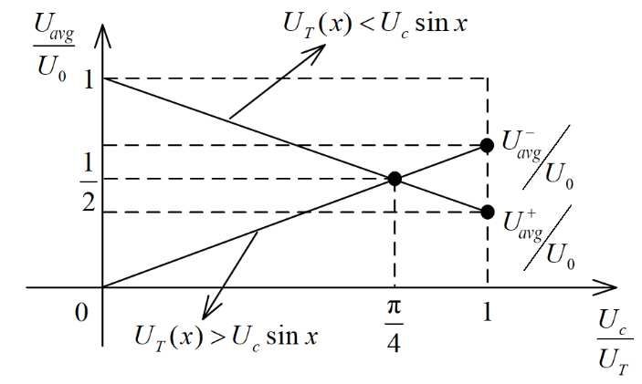
IPDME 2020                                                                                                      IOP Publishing
Journal of Physics: Conference Series                         1753 (2021) 012015          doi:10.1088/1742-6596/1753/1/012015

Linear voltage regulation in DC-to-DC converters

                     A P Veselovskiy1, L I Kosareva2 and S G Zverev1
                     1
                       Peter the Great St. Petersburg Polytechnic University, 29, Polytechnicheskaya str.,
                     Saint Petersburg, 195251, Russia
                     2
                       Military Institute (engineering and technical) VA MTO named after Army General
                     A.V. Khrulev, 22, Zakharyevskaya str., Saint Petersburg, 191123, Russia

                     E-mail: a_veselovskiy@mail.ru, kosareval52@mail.ru, s.zverev@spbstu.ru

                     Abstract. The article deals with the most dynamically developing branch of power electronics
                     related to solving tasks of voltage regulation in DC-to-DC converters. Linear regulation of the
                     output voltage is carried out using pulse-width modulation. A linear regulatory characteristic is
                     obtained over the entire control range from zero to maximum values. The formula of the output
                     voltage regulation characteristic is obtained through a mathematical model of a pulse-width
                     control method with a variable pulse width.

1. Introduction
The wide variety of control systems can be classified by the most important distinguishing features. At
the heart of the functions performed by control systems are the requirements for the processes,
implemented by technological installations with specified parameters of power sources, electric drives,
or power sources of radio-technical devices. Modern factory produced converters include local and
remote control, alphanumeric indicators for displaying input and output voltages, output current,
frequency, accuracy of maintaining various parameters and other data.
    These installations require particularly accurate regulation in open and closed control systems. And
using energy-efficient, controlled electric drive with static electricity converters can improve
efficiency, equipment payback, and production profitability [1,2].
2. Principles of converting DC voltage
To improve the consumer properties of products, we can optimize parameters, increase the working
frequency of conversion, reduce power losses on power elements, and reduce dynamic loads in the
power part of the circuit. Regulation of AC and DC voltages uses pulse-width modulating methods
with varying duty cycle [3–5].
   Pulse-width DC-to-DC converters convert DC voltage to pulse one, the average value of which
needs to be adjusted. The output voltage of these converters (before the output filter), as a rule, has the
form of unipolar pulses (Figure 1).

              Content from this work may be used under the terms of the Creative Commons Attribution 3.0 licence. Any further distribution
              of this work must maintain attribution to the author(s) and the title of the work, journal citation and DOI.
Published under licence by IOP Publishing Ltd                          1
IPDME 2020 IOP Publishing
Journal of Physics: Conference Series 1753 (2021) 012015 doi:10.1088/1742-6596/1753/1/012015
Figure 1. Pulse-width modulation of converters with unipolar pulses of equal duration.
The frequency of conversion depends on the dynamic properties of the switches, of which the
converter is made. Due to the constant value of the supplied voltage at the input of the converter,
natural commutation of the switches (thyristors) is impossible, which requires using fully-controllable
elements (lockable thyristors, transistors). GTO-thyristors allow switching up to 1 kHz, IGBT-
transistors – up to about 10 kHz, field-effect transistors – up to 1 MHz and more [1].
The equation of the regulatory characteristic of the pulse-width converter with unipolar and equal
in duration pulses (unipolar modulation), is determined by the degree C of regulation of the output
voltage:
U out 1 tи tи
C= =
U in TU in
0
U in dt =
T
.
An essential point in the converters of DC voltage is the desired linear dependence of output
voltage on the control effect. The peculiarity of dependence = ( ) in pulse-width
modulation (PWM) of voltage is the non-linearity of the output characteristic [6–16]. Regulatory
performance in this mode of regulation is steeply falling, making it difficult to develop regulators
when using microprocessors. Linearity of the characteristic is a huge advantage of the converter,
ensuring optimal construction of devices of automatic process control in output circuits of rectifiers.
We have developed the method of modulated pulse-width control of the power elements of the
converter with changes in the duration of power pulses, allowing to obtain a linear dependence of
output voltage on the control sinusoidal voltage.
Partial linearity of the regulatory characteristics of a controlled rectifier can be obtained using
PWM when changing the control angle α according to the arccosine dependence [17].
The authors proposed a method of regulating the output voltage of PWM, allowing to obtain linear
regulatory characteristic in the range of 0 to 1.
3. Mathematical description of the proposed linear pulse-width regulation method
The control scheme contains a sinusoidal voltage generator and a triangular pulse generator. Positive
half-sinusoid u ( x) = U с sinx (Uc is the amplitude) over the range of 0 to π corresponds to m
triangular pulses. The limits of pulses are lines lk, the equations of which are described by the general
formula:
k −1 m 1 + (−1) k −1
u k ( x) = (−1) 2U т x − k + , x ∈ [ x k −1 , x k ] , k = 1, 2, … , 2m,
π 2
where UТ is the amplitude of triangular pulses (see Figure 2а), and abscissas of the splitting points of
the [0, π] range are defined by the formula:
2IPDME 2020 IOP Publishing
Journal of Physics: Conference Series 1753 (2021) 012015 doi:10.1088/1742-6596/1753/1/012015
πk
xk = . (1)
2m
Pulse-width modulation is carried out as follows: the DC signal of duration π is broken into
rectangular pulses in accordance with the condition: constant voltage U0 is broken into a number of
ranges with the presence or absence of voltage by points of intersection ξk (k = 1, 2, … , 2m) of
triangular pulses with a sinusoidal curve. Meanwhile, voltage will be present in the ranges where the
sine graph lies above (Figure 2b) or, conversely, below (Figure 2c) the triangular pulses.
Figure 2. Intersections of the sinusoidal voltage curve with m triangular pulses (a);
a sequence of rectangular pulses satisfying the condition uТ(x) < Ucsinx (b); uТ(x) > Ucsinx (c)
Rectangular pulses, therefore, are determined in the case of uТ(x) < Uс sinx by the formula:
3IPDME 2020 IOP Publishing
Journal of Physics: Conference Series 1753 (2021) 012015 doi:10.1088/1742-6596/1753/1/012015
m
0U , x ∈ U [ξ 2k , ξ 2 k +1 ],
− k =1
uп ( x) = m
(2)
0, x ∉ [ξ , ξ ]
U
k =1
2k 2 k +1
and in the case of uТ(x) > Uс sinx – by the formula:
m
U 0 , x ∈ U [ξ 2 k −1 , ξ 2 k ],
+ k =1
uп ( x) = m
(3)
0, x ∉ [ξ , ξ ].
U
k =1
2 k −1 2k
It is not possible to analytically obtain the abscissas ξk of the points Mk where straight lines lk cross
the sinusoidal curve u ( x) = U с sinx , so we will do the following:
As a point of crossing of the sinusoidal curve u ( x) = U с sinx and straight line lk, we will take the
point lying on this straight line (we will call it Nk),) the abscissa of which will be δk, and its ordinate
y(δk) we will set as the arithmetic average of the values of the function u ( x) = U с sinx on the edges of
where the straight line lk, is defined, i.e. at xk-1 and xk::
u ( x k −1 ) + u ( x k ) 1
у (δ k ) = = (U с sinx k −1 + U с sinx k ) .
2 2
Substituting expressions for xk-1 and xk from (1), we obtain:
π π( 2k − 1)
у (δ k ) = U с cos ⋅ sin . (4)
4m 4m
Coordinates of the point N k (δ k , у (δ k )) satisfy the equation of the straight line lk .
m 1 + (−1) k −1
y (δ k ) = (−1) k −1 2U т δ k − k + . (5)
π 2
By equating right parts of the formulas (4) and (5), we will get the expression for δk:
U π π(2k − 1) 1 + (−1) k −1 π
δ k = (−1) k −1 с cos sin +k − . (6)
2U т 4m 4m 2 m
Since the boundaries of the rectangular pulses are defined by points δk (5) instead of points ξk, the
formulas (2) and (3) that determine the sequence of these impulses will also change:
for the case uT(x) < Uc sinx
4IPDME 2020 IOP Publishing
Journal of Physics: Conference Series 1753 (2021) 012015 doi:10.1088/1742-6596/1753/1/012015
m
0U , x ∈ U [δ 2 k , δ 2k +1 ],
− k =1
u п ( x) = m
(7)
0, x ∉ [δ , δ ]
U
k =1
2k 2 k +1
and for the case uT(x) > Uc sinx
m
U 0 , x ∈ U [δ 2 k −1 , δ 2 k ],
+ k =1
uп ( x) = m
(8)
0, x ∉ [δ , δ ].
U
k =1
2 k −1 2k
Now we will calculate the average voltage for each case:
1. uT(x) < Uc sinx (formula (7)).
π δ 2 k +1
1 − 1 m U0 m
U −
= u п ( x)dx = δ U 0 dx = π (δ 2 k +1 − δ 2k ) =
π0 π k =1
avg
2k
k =1
U 0U с π π
= cos 2 ⋅ tg -1 .
Uтm 4m 2m
π π π
For m >> 1: cos
→1 , tg ≈ and the formula takes on the form of:
4m 2m 2m
− 2U 0U с
U avg = . (9)
πU т
2. uT(x) > Uc sinx (formula (8).
π δ
1 1 m 2k U m
U +
= u п+ ( x)dx = U 0 dx = 0 (δ − δ 2 k −1 ) ,
π0 π k =1 δ2 k −1 π
avg 2k
k =1
+ 2U 0U с
U avg = U0 − . (10)
πU т
On Figure 3 we present the regulatory characteristic (9) and (10) of the converter derived from this
method of regulation.
5IPDME 2020 IOP Publishing
Journal of Physics: Conference Series 1753 (2021) 012015 doi:10.1088/1742-6596/1753/1/012015
Figure 3. Regulatory characteristic of the converter
According to this regulatory characteristic, our method allows to regulate the DC-to-DC converter
voltage output linearly in the entire range of 0 to 1.
Computer simulation
Computer simulation was done in the MatLab Simulink environment. A diagram of our model
including a measuring device and a display is shown in Figure 4.
Figure 4. Simulation model of a voltage regulator
built in the MatLab Simulink software package
The results of computer simulations are shown in table 1.
Columns 4 and 5 show the obtained average voltage values of rectangular pulses with varying duty
cycle depending on the amplitude of the sinusoidal voltage under two conditions.
Columns 2 and 3 show the results of theoretical calculations performed according to formulas (9)
and (10), respectively.
6IPDME 2020 IOP Publishing
Journal of Physics: Conference Series 1753 (2021) 012015 doi:10.1088/1742-6596/1753/1/012015
Table 1. Results of theoretical calculation and computer simulation
Uavg (theory) Uavg (model)
Uc
uT(x) > Uc sinx uT(x) < Uc sinx uT(x) > Uc sinx uT(x) < Uc sinx
1 2 3 4 5
0 0 100 0 100
0.1 6.3662 93.634 6.39 93.61
0.2 12.732 87.268 12.79 87.22
0.3 19.099 80.901 19.18 80.82
0.4 25.465 74.535 25.57 74.43
0.5 31.831 68.169 31.96 68.4
0.6 38.197 61.803 38.36 61.64
0.7 44.563 55.437 44.75 55.25
0.8 50.93 49.07 51.14 48.86
0.9 57.296 42.704 57.54 42.16
1 63.662 36.338
Comparing the results of calculation and computer simulation, we should note their minimal
discrepancy (within 1...2%).
Figure 5 shows the graphs of the regulatory characteristics plotted using the simulation data.
120
100
uT(x) < Uc sinx
80
Uavg, V
60
40
20
uT(x) > Uc sinx
0
0 0.2 0.4 0.6 0.8 1
Uc, V
Figure 5. Regulatory characteristics of the DC-to-DC converter obtained through computer
simulation
Similarly to the calculated data, the simulation results reflect the linearity of the regulatory
characteristic.
4. Conclusion
As a result of using the PWM method, the regulatory characteristics of DC voltage become linear and
allow for voltage regulation from zero to maximum values. At the same time, it is much easier to use
microprocessor technology to make such voltage regulators. Results of the developed algorithm of the
control device utilizing the PWM method can find broad use in power electronics, electric drives, and
other areas.
This research work was supported by the Academic Excellence Project 5-100 proposed by Peter the
Great St. Petersburg Polytechnic University.
7IPDME 2020 IOP Publishing
Journal of Physics: Conference Series 1753 (2021) 012015 doi:10.1088/1742-6596/1753/1/012015
References
[1] Semenov B Y 2011 Power electronics: Professional solutions (Moscow: Solon-Press)
[2] Sokolovsky G G 2006 AC electric drives with frequency regulation (Moscow: Academia)
[3] Veselovskiy A P, Budko P A, Vinogradenko A M and Kosareva L I 2018 Implementation of the
way of converting AC voltage Problems of technical support of troops in modern conditions: theses of
reports III intercollegiate NPC (St. Petersburg, Military Academy of Communications) pp 172-176
[4] Budko P A, Veselovskiy A P, Vinogradenko A M and Kosareva L I 2018 Voltage regulation in
converters of high-frequency pulses with varying duty cycles Mechatronics, automation, control 8
(19) 516–522 DOI: 10.17587/mau.19.516-522
[5] Voytyuk I N, Zamyatina E N and Zamyatin E O 2019 Increasing the energy efficiency of an
enterprise by point compensating of power quality distortions Proceedings of the International
Scientific Conference on Energy, Environmental and Construction Engineering (EECE-2019)
[6] Romash E M, Drabovich Y I, Yurchenko N N and Shevchenko P N 1988 High-frequency
transistor converters (Moscow: Radio and communication)
[7] Abraham L, Heumann K, Koppelmann F 1964 Wechselrichter fur Dzehzahlsteurung von
Kafiglaufermotoren AEG–Mitt. 2 89-106
[8] Volkov A G 2014 Mathematical model of AC-AC converter without passive elements in DC-
link Source of the Document International Conference of Young Specialists on Mi-
cro/Nanotechnologies and Electron Devices (EDM 2014) 403-407
[9] Shklyarskiy Y E, Shklyarskiy A Y and Zamyatin E O 2019 Analysis of distortion-related elec-
tric power losses in aluminum industry Tsvetnye Metally 4 84-91
[10] Vinogradenko A M, Veselovskiy A P, Vzesniewski S V and Galvas A V 2018 The way and the
synchronization of voltage control systems Practical power electronics 2 (70) 53-55
[11] Skamyin A N and Dobush V S 2018 Analysis of nonlinear load influence on operation of
compensating devices IOP Conference Series: Earth and Environmental Science 194 (5) 052023 DOI:
10.1088/1755-1315/194/5/052023.
[12] Kopteva A V, Starshaya V V, Malarev V I and Koptev V Yu 2019 Improving the ef-ficiency of
petroleum transport systems by operative monitoring of oil flows and detection of ille-gal incuts
Topical Issues of Rational Use of Natural Resources Proceedings of the XV International Forum-
Contest of Students and Young Researchers under the auspices of UNESCO (1) (St. Petersburg Mining
University, Russia) pp 406-415
[13] Batueva D and Shklyarskiy J 2019 Increasing Efficiency of Using Wind Diesel Complexes
through Intellectual Forecasting Power Consumption IEEE Conference of Russian Young Re-
searchers in Electrical and Electronic Engineering (EIConRus) pp 434-436 Doi:
10.1109/EIConRus.2019.8657158
[14] Savard C and Iakovleva E V 2019 A suggested improvement for small autonomous energy
system reliability by reducing heat and excess charges Batteries 5(1) 29 Doi:
10.1109/EIConRus.2019.8657097.
[15] Chmilenko F V and Rastvorova I I 2018 Improvement of quality of aluminum ingots at elec-
tromagnetic processing Journal of Physics: Conference Series 1118(1) 012030
[16] Dobush V, Belsky A and Skamyin A 2020 Electrical Complex for Autonomous Power Supply
of Oil Leakage Detection Systems in Pipelines Journal of Physics: Conference Series 1441 Doi:
012021. 10.1088/1742-6596/1441/1/012021
[17] Veselovskiy A P, Budko P A, Buryanov O N and Vinogradenko A M 2017 Features of the
systems of control of ventral converters Problems of technical support of troops in modern con-
ditions: theses of reports II intercollegiate NPC (St. Petersburg, Military Academy of Communica-
tions, 2017) pp 150–154
8You can also read