Local Carbon Policy José-Luis Cruz and Esteban Rossi-Hansberg - Becker Friedman Institute
←
→
Page content transcription
If your browser does not render page correctly, please read the page content below
WORKING PAPER · NO. 2022-57

Local Carbon Policy
José-Luis Cruz and Esteban Rossi-Hansberg
MAY 2022

                                                       5757 S. University Ave.
                             An Affiliated Center of
                                                           Chicago, IL 60637
                                                        Main: 773.702.5599
                                                            bfi.uchicago.edu
Local Carbon Policy*
José-Luis Cruz Esteban Rossi-Hansberg
Princeton University University of Chicago
May 2, 2022
Abstract
We study local carbon policy to address the consequences of climate change. Standard analysis suggests
that the social cost of carbon determines optimal carbon policy. We start by using the spatial integrated
assessment model in Cruz and Rossi-Hansberg (2021) to measure the local social monetary cost of CO2
emissions: the Local Social Cost of Carbon (LSCC). Although the largest welfare costs from global warming
are concentrated in the warmest parts of the developing world, adjusting for the local marginal utility of
income implies that the LSCC peaks in warm and high-income regions like the southern parts of the U.S.
and Europe, as well as Australia. We then proceed to study the effect of the actual carbon reduction pledges
in the Paris Agreement and the progress they can make in implementing the expressed goal of keeping
global temperature increases below 2◦ C. We find that although the distribution of pledges is roughly in
line with the LSCC, their magnitude is largely insufficient to achieve its goals. The required carbon taxes
necessary to keep temperatures below 2◦ C over the current century are an order of magnitude higher
and involve large implicit inter-temporal transfers. Increasing the elasticity of substitution across energy
sources is important to reduce the carbon taxes necessary to achieve warming goals.
* Cruz: jlca@princeton.edu. Rossi-Hansberg: earossih@uchicago.edu. We thank Jordan Rosenthal-Kay for helpful comments.
11 Introduction
The impact of temperature increases caused by CO2 emissions is, and will be, heterogeneous across loca-
tions of the world. Regions in Central Africa or India will experience large losses in welfare over the next
few centuries while regions in the northern parts of Canada, Europe, or Russia could benefit from rising
temperatures. Hence, from a particular region’s perspective, the social need for climate policy can vary
substantially. What are the incentives to impose carbon taxes across locations of the world? How are these
incentives related to actual pledges in the Paris Agreement? What are the implications of these pledges for
aggregate temperatures and the economies of different regions across the globe? In this paper we explore
these questions using the spatial integrated assessment model in Cruz and Rossi-Hansberg (2021).
The social cost of carbon has become the standard measure to benchmark the magnitude of the carbon
taxes needed to implement optimal carbon policy. It measures the social cost in U.S. dollars of adding a
ton of CO2 to the atmosphere. If we were able to measure this social cost accurately, standard Pigouvian
logic tells us that the optimal tax should be such that the price of carbon is equal to this social cost. Since
carbon emissions are a global externality there is, at least in principle, a world’s social cost of carbon that
takes into account all the implications of the additional ton of CO2 throughout the world and over time.
The price of carbon should then be set at this price, everywhere. Of course, this logic is correct only from a
global planner’s point of view, where the planner puts equal weights across individuals. Its implementation
requires transfers from the regions that are less affected, or positively affected, by CO2 emissions to the
countries that are negatively affected. In practice, countries and regions tend to consider the implications of
climate change for themselves, not for the whole world. Their incentives to pursue climate policy via carbon
taxes, reflect their own evaluation of the social cost of carbon, not necessarily the world’s. To understand
what these incentives are, we start by computing the Local Social Cost of Carbon (LSCC) at a resolution of
1◦ × 1◦ across the globe.
The LSCC is determined by the local willingness to pay for the effects caused by an additional ton of
CO2 emissions. It can be decomposed in two parts: the welfare cost of the additional carbon emissions and
the inverse of the marginal utility of income. The latter component allows us to express the LSCC in dollars
per ton of CO2 , rather than utils per ton of CO2 . In Cruz and Rossi-Hansberg (2021), we have argued that
the welfare costs of climate change are extremely heterogeneous across locations due to the different local
temperature effects from increases in average world temperatures, from differential effects on amenities,
productivity, and natality of changes in local temperatures, and from the differential cost of migration and
trade across regions of the world. Measuring these welfare costs requires a framework encompassing the
full range of impacts of CO2 emissions, from the implied increases in local temperatures to their effects
on regional economies, accounting for the costly mobility of agents, changes in trade patterns, and future
local investments and growth. We employ the framework developed by Cruz and Rossi-Hansberg (2021)
as it allows us to compute the LSCC at a fine level of resolution and accounts for a number of adaptation
2mechanisms over time.
The welfare implications from global warming are particularly large for developing countries close to
the Equator, where temperatures are higher. Central Africa and parts of Central and South America, as
well as South East Asia are particularly negatively affected. The LSCC combines this heterogeneity with
the spatial heterogeneity in the inverse of the marginal utility of income. This value is naturally small in
today’s rich regions since people obtain more of their welfare from consumption rather than from amenities
or migration.1 The division of these two effects determines the LSCC.
The resulting geography of the LSCC is very different than the geography of the welfare losses from
additional emissions due to the marginal utility component. This component increases the LSCC in pro-
ductive countries relative to their overall welfare losses from warming, and has the opposite effect in devel-
oping countries which are less productive. Therefore, the LSCC is high in the warmest places of rich areas,
like the south of Europe or the U.S. and Australia, and in middle income countries like Brazil, Mexico, and
South Africa. In Northern Canada and Russia, the effect of welfare makes the LSCC negative in the baseline
business as usual scenario. In more extreme scenarios, the LSCC is positive everywhere but its geography is
similar.
Of course, any calculation of the social cost of carbon requires taking a stand on the relevant inter-
temporal discount factor. In fact, the global social cost of carbon, as well as the LSCC, are extremely sensitive
to the value of this discount factor. As we move the discount factor from 0.965 to 0.97, the global social cost
of carbon goes from about 5 to 40 dollars ($) per ton of CO2 2 . The permanent growth rate in the baseline
scenario is 2.97%, so we cannot increase it much further. Regions in the upper 1% of the distribution have
much larger LSCC, ranging from about 30$ to 120$ as we vary the discount factor.
We then turn to studying local carbon policy and its effects. Our starting point is the geography of
the LSCC which determines the local incentives to tax carbon if the location could unilaterally determine
global policy. Of course, each region setting carbon prices at the LSCC level is not necessarily the optimal
policy since it only considers each region’s own social cost and does not internalize the policy actions of
others. Unfortunately, we cannot solve the planner’s problem and determine optimal local carbon policy
directly since the dynamics of the model are too complex. Furthermore, because the equilibrium spatial
distribution of economic activity is not optimal due to static and dynamic externalities, the carbon taxes and
the transfers resulting from the tax revenue rebates can affect the efficiency of the spatial distribution and
therefore the cost of the tax. This makes the optimal policy potentially spatially heterogeneous and likely
complex. Instead, here we simply compare the LSCC to the actual local pledges in the Paris Agreement
for the period 2022 to 2030. The magnitude of these pledges is large in many of the areas where the LSCC
cost is also large, so both policies have a similar, although by no means identical, spatial distribution. In
1 In our model utility is linear in the consumption aggregate of varieties. However, the ability to move implies that utility equalizes
across locations up to moving costs. Hence, amenities, which determine the marginal utility of income, are lower in productive places
across location with small moving costs.
2 Throughout the paper nominal values are expressed in year 2000 dollars.
3particular, Europe and the U.S. made relatively large pledges. China did too, although its LSCC is small
except in its more productive regions in the eastern coast.
In order to analyze the impact of the Paris Agreement, we first calculate the carbon tax equivalent of the
carbon emission reduction pledge for a partition of the world in nine regions. We then study the effect of
imposing these carbon taxes unilaterally. We find that CO2 leakage can be positive or negative depending
on the region. When regions that are large and rich, like the U.S. and Europe, impose unilateral carbon
taxes their economies shrink. Their costs grow relative to other countries, which results in out-migration
and lower levels of investments. The rest of the world grows, but the additional production concentrates in
the most productive areas with high carbon prices. The result is a small increase in real GDP in the rest of
the world, but a net reduction in emissions. In contrast, when relatively low income per capita countries,
like China, impose carbon taxes, leakage is positive and the rest of the world ends up emitting more CO2 .
We also analyze the case in which all regions implement their pledges in the form of carbon taxes simul-
taneously. The required carbon taxes are naturally larger in this case, since policy action leads to smaller
reductions in local GDP due to the simultaneous actions of others. Overall, we find that these pledges re-
duce carbon emissions little relative to the baseline and that the effect on temperatures is small. Hence, they
are not sufficient to keep temperature increases below 2◦ C relative to pre-industrial levels by 2050 and far
from the level necessary to keep temperatures below 2◦ C by 2100. If all countries implement carbon taxes
equivalent to their 2030 pledges permanently, temperatures by 2100 reach levels of more than 4◦ C relative
to pre-industrial levels. Keeping the distribution of CO2 emissions in the Paris Agreement constant, we
estimate that the policy necessary to keep temperatures below 2◦ C by 2050 is, on average, more than two
times larger than the policy required to reach the Paris Agreement. The policies needed to keep tempera-
tures below 2◦ C by 2100 are an order of magnitude larger, and perhaps unrealistic. The average tax per ton
of CO2 would need to be as large as 500$. Such a policy implies a large inter-temporal transfer between
current and future generations. World real GDP falls as much as 10% at impact, recovers and becomes
larger than without the carbon policy only by 2150.
Carbon taxes are relatively ineffective at reducing carbon emissions because they tend to delay, rather
than eliminate, carbon use. The reason is that carbon-based energy costs increase as the world uses more
carbon. Larger taxes reduce use, and therefore delay this process. Cruz and Rossi-Hansberg (2021) explains
this mechanism in detail. As carbon becomes more expensive due to carbon taxes, the world uses less
carbon-based energy, but it does not eliminate its use completely since substitution is costly (particularly
in certain industries and uses). We model this substitution using a constant elasticity of substitution in the
energy production process with fossil fuels and clean energy as inputs. The elasticity of substitution in this
function is crucial in determining the timing of carbon use and the effectiveness of the tax in delaying its
use. We use a value of 1.6 in our baseline scenario but present results also for the case when it takes the
value of 3. Of course, this elasticity is partly a policy variable. Policy can incentivize the use of equipment
that can more easily substitute between both types of fuel, for example, electric cars and buses.
4Our paper is the first one to discuss the LSCC at such a high spatial resolution, considering costly migra-
tion, costly trade, and local investments in a model with a fully fledged economic geography and a rich set
of agglomeration and congestion forces. Tol (2011) surveys the literature on the economic impacts of climate
change and the different methods employed to estimate the impact of climate change on human welfare.
Nordhaus (2017) computes the social cost of carbon in the global economy. Carleton and Greenstone (2021)
provides a set of guidelines to compute the global social cost of carbon. Carleton et al. (2022) estimate age-
specific mortality-temperature relationships and compute a mortality partial social cost of carbon. Hassler
et al. (2020) discusses carbon pricing in the Swedish context.
The rest of the paper is structured as follows. Section 2 outlines the key elements of the economic and
climate model and its quantification. Section 3 quantifies the LSCC and describes how it varies across dam-
age levels and discount factors. Section 4 discusses the efficiency of the Paris Agreement to limit warming
and explores different combinations of environmental policies to reduce the temperature path. Section 5
concludes.
2 Model and Quantification
In order to analyze the local effects of environmental policies we need a spatial dynamic model of global
warming with a realistic geography. Cruz and Rossi-Hansberg (2021) develops such a framework. It ex-
tends the model in Desmet et al. (2018) to incorporate endogenous population growth and energy as an
input of production. It also incorporates a climate component through a carbon cycle, and the effect of the
implied temperature changes on amenities, productivity, and natality rates. Instead of presenting the full
model, here we limit ourselves to briefly describe the main elements of the model and its quantification.
We refer the reader to the paper for a technical description.
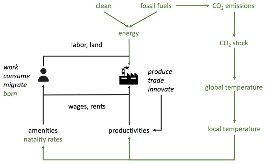
Figure 1 describes the workings of the model. The components in black denote the baseline model from
Desmet et al. (2018) and the components in green represent the additions by Cruz and Rossi-Hansberg
(2021). We divide the land mass of the world in 17,048 locations, with a resolution of 1◦ × 1◦ . Each location
is unique in terms of its amenities, productivity, geography, as measured by its bilateral transport costs to
all other regions and the migration frictions to enter them, as well as its climate conditions. Agents derive
utility from consuming a continuum of a fixed set of varieties and from common and idiosyncratic amenities
in their location of residence. If agents move, they pay migration costs in the form of a permanent utility
discount that is log-linear in an origin and a destination effect. Agents supply land and labor inelatically
to firms and receive the corresponding payments. Every period they face a consumption decision and a
migration decision. The natality rate (birth minus death rate) at a location is determined by a location’s
income and temperature in order to capture demographic transitions and the effect that temperature can
have on mortality.
Firms in a location use land, labor, and energy as inputs to produce specific varieties that they trade
5Figure 1: Model description
with other locations subject to iceberg transport costs. They use a constant-returns-to-scale Cobb-Douglas
technology in these three inputs. They generate the energy input by combining fossil fuels and clean energy
sources using a constant elasticity of substitution technology with elasticity given by ϵ. Firm’s productivity
is idiosyncratic and drawn from a Fréchet distribution. The level of this distribution is determined dy-
namically by local production externalities, technology diffusion from other locations, and the firm’s own
innovation decisions. Firms can shift the distribution from which they draw their technology every period
by paying an innovation cost. They compete to produce in a given location through competitive bidding.
They innovate optimally to gain the bid, but end up with zero profits since they transfer all the surplus
from innovation to the fixed factor, namely, land. Local residents are the owners of land and receive all
land rents.
The result is a model in which congestion forces, which are determined by negative externalities of con-
gestion in amenities, idiosyncratic preferences for location, and having land (a fixed factor) as an input in
production, balance with agglomeration forces, given by local externalities, as well as dynamic agglomera-
tion forces coming from the firm’s investment decisions which are monotone in a firm’s market size. Firm
market size is determined by the distribution of expenditures discounted by the relevant transport costs.
The presence of technology diffusion and externalities in productivity and amenities implies that the equi-
librium allocation is not efficient, even without considering the climate externality. The equilibrium of the
model is unique under some parameter restrictions that are satisfied in the quantification and amount to
congestion forces ultimately dominating agglomeration forces.
The combustion of fossil fuels to generate the energy used by firms releases CO2 emissions into the
atmosphere, where they accumulate and warm up the Earth. We use the model of the carbon cycle in IPCC
(2013) which determines the evolution of global temperature given firm’s emissions. We set the prices of
6fossil fuels and clean energy in the year 2015 to target the observed CO2 emissions and use of clean sources
at the country-level. The local prices of clean energy and fossil fuels evolve with the world’s technology
frontier, with elasticities that replicate the evolution of their use in the world economy. The local price of
fossil fuels also depends on extraction cost which are low when fossil fuels are abundant, but rise sharply
as they become exhausted (as in Bauer et al., 2017). Local temperature variation is determined by aggregate
temperature variation through a constant local down-scaling factor, as suggested by Mitchell (2003).
Changes in local temperatures affect amenities and productivity through damage functions estimated
in Cruz and Rossi-Hansberg (2021). They determine the different semi-elasticities of changes in local tem-
perature on amenities and productivity, conditional on the level of temperatures. They are estimated using
a panel of model-implied local amenities and productivity over four years that control for all the adaptation
mechanisms incorporated in the model. As such, they represent the effect of temperature on fundamentals,
not on individual or firm reactions. The causal effect of temperature on amenities and productivity are
estimated using a panel fixed effect empirical specification with regional trends. The estimated damage
functions show that the semi-elasticity of temperature on amenities is about 2.5% in the coldest regions of
the world, declines continuously and is negative and about the same absolute magnitude in the warmest
places. Namely, in the warmest places on Earth a 1◦ C increase in local temperature decreases amenities by
2.5%. The damage function for productivity has a similar shape although the effects are larger and asym-
metric with reductions of more than 10% in productivity in response to a 1◦ C increase in temperatures in
the warmest regions. Finally, we specify local natality rates as a declining function of real income and as
a bell-shaped function of temperature. Hence, when temperatures are extreme, natality rates are low and
they are maximized in temperate climates.
The model quantification relies on data on the geographic distribution of population and income from
G-Econ, the Human Development Index, and bilateral transport costs to construct measures of local pro-
ductivity and local amenities that exactly rationalize this data through our framework. In addition, we
estimate mobility frictions to match net local changes in population between 2000 and 2005. With the quan-
tified model in hand, we can compute the cell-level welfare impact of increases in CO2 emissions as well as
the cell-level marginal utility of income, which allows us to measure the LSCC. We can also impose carbon
taxes in any cell of the world and measure their impact.
3 The Local Social Cost of Carbon
The Social Cost of Carbon (SCC) is a central concept for understanding environmental policy, as it repre-
sents the global monetized value of all present and future net damages associated with a one ton increase
in CO2 emissions (Carleton and Greenstone, 2021). Therefore, its quantification depends on how compre-
hensive are the models to calculate it. We include the main channels through which CO2 emissions can
affect individuals, allow for several adaptation mechanisms, and do the proper aggregation from local to
7global effects. One limitation is that we only measure the part of the SCC associated with local temperature
increases, but do not include the part associated with other related phenomena, like coastal flooding.3 The
cost of those effects should be added to the costs we compute here. Although we present implications of
our model and a quantification of the SCC, we are more interested in the Local SCC (LSCC). The concept is
similar, and it is still calculated in a global model, but it considers the monetized value of all local damages.
Thus, it represents the extent to which global CO2 emissions damage a particular location and, therefore,
the level at which these regions should want to set a global carbon price. Of course, in actual negotiations,
countries will not necessary want to impose taxes that set the local price at this level, since they realize that
there might be leakage to other regions if they do not impose a similar tax. Nevertheless, it does measure
the local social incentives to price carbon.
We define the LSCC of region r at period t as
,
∂Wt (r) ∂Wt (r)
LSCCt (r) = − , (1)
∂Etf ∂wt (r)
where
∞
X
Wt (r) = β t−ℓ uℓ (r), (2)
ℓ=t
denotes local per capita welfare, ut (r) local per capita utility, wt (r) local per capita nominal income, Etf
global emissions of CO2 , and β the discount factor (which we set to β = 0.965 in our baseline simula-
tion since the balance growth path features real GDP growth of about 3%). The numerator represents the
marginal local welfare impact of additional global carbon emissions and the denominator represents the
marginal local welfare impact of an additional U.S. dollar adjusted by Purchasing Power Parity.4 In sum,
the LSCC equals the economic impact of a unit of emissions in terms of t-period nominal income.
We compute the LSCC using a discrete approximation. Specifically, we consider our business as usual
baseline path of emissions and increase the carbon dioxide emissions by one ton in the year 2022. Then,
we simulate the economy forward for four centuries and compute local welfare in 2022. We then repeat
the exercise absent the pulse of carbon dioxide. The difference in welfare between these two scenarios
approximates the numerator of equation (1). As for the denominator of equation (1), in order to express
the LSCC in U.S. dollars adjusted by Purchasing Power Parities, we consider an increase in local income
in 2022 assuming that it only affects current utility with no effects afterwards. More precisely, when local
wage rises, we allow for the adjustment in prices and population, but take the fundamentals of the model
(i.e., productivity, amenities, land endowment, energy prices, and trade and migration costs) as given.
3 See Desmet et al. (2021) for an evaluation of coastal flooding in a related framework.
4 In our model, conditional on the level of amenities and migration costs, utility is linear in real income. We could easily extend
the model to incorporate a period utility function that is concave in real income. This would increase the dispersion in the spatial and
inter-temporal distribution of the marginal utility of income.
8Figure 2 displays the spatial distribution of the LSCC. We consider two different scenarios: the baseline
scenario, defined by the point estimates of the damage functions on amenities and productivity described
in the previous section, and the worst-case scenario characterized by the 95% lower confidence interval of
the damage functions.5 We present the LSCC in terms of dollars per metric ton of CO2 ($/tCO2 ).6
Figure 2: Local Social Cost of Carbon in the baseline and worst-case scenario.
In the baseline scenario, the LSCC is positive in the warmest locations of the world and negative in
the Arctic. The highest values of the LSCC are observed in the hottest and richest regions of the world:
Australia, the Arabian Peninsula, and the south of Europe and the United States. All of them are high
income locations that will experience intermediate welfare costs from temperature increases. Even though
lower income locations in Sub Saharan Africa and India are expected to experience the largest welfare losses
from global warming, the LSCC of these places lies between 2$ and 5$ only. The LSCC in the worst-case
scenario exhibits a similar pattern with a larger spatial dispersion and higher average values. On average,
the LSCC takes the values of 5.23$/tCO2 and 14.97$/tCO2 , respectively, where the global average uses as
weights the population shares in the year 2022. Of course, these averages depend heavily on the chosen
discount factor, an issue that has been extensively discussed in the literature (see Carleton and Greenstone,
2021 for a summary) and to which we return below.
The structure of the damage functions suggests that the largest welfare losses in amenities and produc-
tivity occur in the hottest locations of the world. This logic might suggest that the LSCC should also be
higher in the tropical areas and gradually decline in colder locations. However, the spatial distribution
of the LSCC shows the largest values in high income locations that experience negative but not the most
extreme welfare losses. To disentangle the forces shaping the LSCC, we decompose this term into the per-
5 In Appendix B, Figure 11 presents the distribution of the LSCC, Figure 12 displays the LSCC in the best-case scenario, charac-
terized by the 95% higher confidence interval of the damage functions and Table 5 displays the LSCC by country for the baseline and
worst-case scenario and for different discount factors.
6A ton of CO2 contains 0.2727 tons of carbon (tC), so a LSCC of 10$/tCO2 is equivalent to 36.67$/tC.
9centage change in welfare derived from the pulse of CO2 (the welfare component), the monetization from
utils to dollars (the inverse marginal utility or monetization component), and the unit adjustment; namely,
!, !
∆Wt (r)[∆Etf ] ∆ut (r)[∆wt (r)]
LSCCt (r) = −
1 tCO2 1$
! !−1 !
∆Wt (r)[∆Etf ] ∆ut (r)[∆wt (r)] 1$
=− ,
ut (r) ut (r) 1 tCO2
where ∆Wt (r)[∆Etf ] denotes the change in Wt (r) as a result of the change in carbon emissions, Etf , and
∆ut (r)[∆wt (r)] the change in utility as a result of the change in income, wt (r).7 The left panel of Figure
3 illustrates the percentage change in welfare derived from the pulse of CO2 . The figure resembles the
spatial distribution of welfare losses from global warming (see Figure 8 in Cruz and Rossi-Hansberg, 2021),
as temperature increases have the most pernicious effects in the warmest and poorest locations and the
most favorable effects in northern locations. The highest income regions are at a cusp where the effects are
relatively small, but negative. The right panel of Figure 3 illustrates the monetization, or inverse marginal
utility component, which is related to local wages, local migration costs, and amenities. The main effect is
that a higher level of income is associated with lower marginal utility. That is, a larger increase in income is
required to achieve a given increase in utility. Note that this component is also large in magnitude relative
to the welfare component, and always positive. The balance of these two components implies that the
LSCC is the highest in hot, but also relative rich regions. A good example of this balance is the South of
U.S., where the welfare effects are marked yet not extreme, but where the low marginal utility of income
yields one of the largest LSCCs in the world.
Figure 3: Decomposition of the Local Social Cost of Carbon in the baseline scenario.
Global warming is a protracted phenomenon with long lasting consequences. Hence, the discount factor
7 Appendix A formally derives the monetization component in terms of the wage and utility level.
10we use plays a crucial role in determining the magnitude of the LSCC, although it plays less of a role
in its spatial distribution described in Figures 2 and 3. In our framework, the discount factor has a role
in the aggregation of inter-temporal effects from carbon emissions, but it has no allocative effect since
all decisions ultimately are reversible or are independent of future outcomes. Hence, decisions on the
level of the discount factor are purely decisions on the relevant social welfare function for inter-temporal
aggregation; the choice answers the question, how do we value the welfare of future generations of humans
today? Because our model features permanent growth and the utility function is linear in consumption, β
is bounded by the inverse of the growth rate of real GDP. In the baseline scenario, the growth rate in the
balanced growth path (BGP) of the economy is 2.97%8 and thus the discount factor cannot exceed 0.97.
Future generations will be richer, so we cannot value them too highly and still have well defined present
discounted values.
Figure 4: Local Social Cost of Carbon across percentiles in the baseline and worst-case scenario.
Figure 4 presents the LSCC in the baseline and worst-case scenarios for different values of the discount
factor. The solid line denotes the global population weighted average, which provides a measure of the
global SCC. A global carbon tax should target this level if the welfare criterion is a utilitarian world plan-
ner.9 The shaded areas represent the spatial heterogeneity across regions of the world. Clearly, higher
discount factors rise both the average and the standard deviation of the LSCC. In the baseline scenario,
with a discount factor of β = 0.97, the SCC is 40$ per ton of CO2 emissions. However, this tax is too low for
regions that include about 40% of the population of the world. The highest 1% of population would like a
carbon price of about 115$/tCO2 . Similarly, many locations, in fact 60% of the population since the distri-
bution has a long right tail, would find the 40$/tCO2 carbon price too high according to their LSCC. The
8 The BGP growth rates are 2.98% and 2.96% in the worst-case and best-case scenarios, respectively.
9 Thisis a local argument. As the economy evolves, the global SCC changes, and the optimal global carbon tax would change as
well. Note also that the optimal policy would consider an optimal distribution of tax revenue rebates across space. We rebate the tax
locally, which is not necessarily globally optimal. As discussed in the introduction, we have not develop a methodology to compute
the optimal policy in this framework yet.
11second panel of Figure 4 presents the same graph for the worst-case scenario. Now, the SSC for β = 0.97 is
around 60$/tCO2 , but the LSCC in the regions with the highest values is as large as 190$/tCO2 . As in the
baseline scenario, the skewness in the distribution implies that the average SCC would be too high for the
majority (70%) of people (but also way too low for many others). Clearly, the distribution of the LSCC is
relevant for studies of the political economy of carbon policy.
In light of our findings, we now turn to the analysis of actual carbon policy as reflected in the pledges
embedded in the 2015 Paris Agreement and its stated goal of keeping global temperature increase below
2◦ C relative to pre-industrial levels.
4 Measuring the Impact of the Paris Agreement
In 2015, world leaders at the UN Climate Change Conference (COP21) signed the Paris Agreement, which
has as objective to hold the increase in global average temperature well below 2◦ C relative to pre-industrial
levels and pursue efforts to limit the temperature increase to 1.5◦ (UN, 2015). This goal is linked to a re-
quirement that all countries design plans for climate action, known as nationally determined contributions
(NDCs).10 When countries submit their NDCs, they express their climate goals in an array of different
measures. Therefore, it is challenging to compare what pledges really mean in terms of emission and, ulti-
mately, temperature goals. In order to harmonize and model the diversity of climate goals, we follow King
and van den Bergh (2019). They group NDCs into four categories: 1) Greenhouse gas (GHG) reductions
relative to the emissions of a given year; 2) GHG reductions relative to a projected business as usual sce-
nario; 3) reductions in the intensity of GHG emissions per GDP; and 4) the implementation of projects to
reduce GHG emissions. They normalize the emission pledges by expressing them as the implied emission
reduction relative to emissions in the year 2015.
To simplify the interpretation of our results, in our implementation we aggregate the country-level
pledges into 9 region-level pledges.11 We also limit the scope of the pledges from all greenhouse gases
to only CO2 emissions from fuel combustion. We do so by multiplying the fossil fuel induced CO2 emis-
sions in the year 2015 by the ratio of the pledges for all GHGs in terms of the GHGs in the year 2015.12
Figure 5 compares the observed CO2 emissions in 2015 (yellow green bar), the projected emissions for the
year 2030 in our baseline business as usual scenario (dark green bar), and the Paris Agreement emissions
targets by 2030 (dark cyan bar).
Figure 5 shows that the pledges of China, North America and Europe are the most aggressive, followed
by Asia Pacific, Eastern Europe and Central Asia, and Latin America. The pledges in the Middle East and
10 When preparing NDCs, some countries attached conditions (e.g., financial support or action in other countries) to the implemen-
tation of some measures. In the subsequent analysis, we restrict attention to the unconditional NDCs.
11 Figure 13 in Appendix B illustrates the geographical composition of the regions.
12 We perform this adjustment because our model only models the emissions of carbon dioxide from fuel combustion.
12Figure 5: Paris Agreement Pledges.
Africa are either very small, or do not involve concessions according to our projections. We will implement
these pledges in our model by finding the set of carbon taxes that implements these goals either unilaterally
or collectively when all countries implement the Paris Agreement simultaneously. The second scenario is
probably the most realistic, but the first one helps us discuss carbon leakage and its consequences.
Unilateral Policy We start by consider the unilateral implementation of regional carbon taxes that achieve
the Paris Agreement pledges. For each region of analysis, we find the carbon tax consistent with achieving
the local pledge by 2030 (which requires solving a fixed point numerically). Here, we assume that the rest
of the world introduces no environmental policy. The carbon tax is implemented in 2022 and increases
over time proportionally to the evolution of fossil fuel prices.13 Throughout, we assume that tax revenue is
rebated locally as a lump sum transfer.
The second column of Table 1 presents the carbon taxes, expressed in U.S. dollars per ton of CO2 , re-
quired to unilaterally comply with the Paris Agreement.14 The third and fourth columns present the per-
centage decline in CO2 emissions in the region itself (the Paris Agreement pledge) and in the rest of the
world. The adoption of a carbon tax in a given region might induce more (highlighted in blue) or less
(highlighted in red) emissions in the rest of the world. That is, carbon taxes might yield positive or negative
carbon leakage! In contrast, as is clear from the last two columns, the effect on real GDP in the country that
13 Theprice of fossil fuels in each location is determined as the value that rationalize the local relative consumption of fossil fuels
and clean energy. Thus, local prices represent an aggregation of the prices across different industries and energy sources. For a model
with energy prices at the industry level, see Cruz (2021).
14 Table 6 in Appendix B replicates Table 1 for an elasticity of substitution in the production of energy of ϵ = 3.
13Carbon Tax ∆%CO2 ∆%Real GDP
Region
($/tCO2 ) Own RoW Own RoW
Asia Pacific 6.71 -9.08 -0.03 -1.23 0.06
China 12.28 -21.92 0.69 -2.99 0.29
Eastern Europe and Central Asia 5.06 -12.50 0.05 -1.75 0.03
Latin America and Caribbean 17.61 -16.73 -0.04 -2.24 0.06
Middle East and North Africa 0 0 0 0 0
Northern America 10.45 -40.48 -0.58 -5.78 0.08
South Asia 0 0 0 0 0
Sub Saharan Africa 60.98 -14.94 0.19 -2.05 0.11
Europe 16.31 -30.58 -0.72 -4.16 0.09
Table 1: Unilateral carbon taxes to achieve the Paris Agreement pledges and their consequences.
imposes the policy is always negative, and it is always positive for other countries.
The conventional argument for carbon leakage indicates that higher carbon taxes abroad make domestic
fossil fuels relatively cheaper, leading to an increase in CO2 emissions and positive leakage. This effect
dominates when China, Eastern Europe and Central Asia, and Sub Saharan Africa impose a unilateral tax.
However, the substitution effect of a carbon tax does not comprise the total effect. In addition, a higher
carbon tax shifts production to regions that have different productivity and relative cost of carbon fuels. If
the shift implies that production in the rest of the world is now concentrated in more productive regions
(that use less inputs per unit of output) or regions with higher relative carbon prices, the result can be a
reduction in emission even if the rest of the world produces more real output. This second effect dominates
for rich countries, like the U.S. or Europe. In these countries, the carbon tax shifts production to other
regions of the world that are also very productive but that have relatively large fossil fuel costs.
Multilateral Policy: Implementing the Paris Agreement We now proceed to study the coordinated im-
plementation of the Paris Agreement. In practice, we compute the set of carbon taxes that simultaneously
meet the pledges in each region of the world. This requires solving numerically for a fixed point in the
model implied carbon emissions for our 9 regions simultaneously. According to Table 2, a global average
carbon tax of 12.21$/tCO2 is required to achieve the pledges in the Paris Agreement. The largest carbon
taxes are observed in North America and Europe, as these regions promised the largest declines in CO2
emissions by 2030. The U.S. would need to implement a carbon tax of 47$ per ton of CO2 . Europe would
need to implement additional carbon taxes of 31$ per ton of CO2 . Note that these taxes are required on top
of the policy already in place in the business as usual scenario. China would need to introduce a smaller tax
of 20$ per ton of CO2 . For all countries, except Sub Saharan Africa, the carbon tax required to achieve the
Paris Agreement pledges in the simultaneous case is substantially larger than in the unilateral case, since
real GDP in locations that implement carbon taxes declines less when other countries impose carbon taxes
as well.
The results above depend crucially on the elasticity of substitution between clean energy sources and
14fossil fuels in the production function of the energy input, ϵ. Although in Cruz and Rossi-Hansberg (2021)
we treat this elasticity as fixed, it is natural to think that its value can change with policy or with the
characteristics of the capital stock. For example, if the car and bus fleet is electric, the energy it uses is
perfectly elastic in fossil or clean energy sources. In contrast, gasoline base transportation requires fossil
fuels and therefore is perfectly inelastic. The value we use in our baseline study, ϵ = 1.6, is based on current
evidence given installed technology,15 but it is easy to envision that innovations or future investments can
increase this elasticity substantially. Hence, in Table 2, we present the required taxes to implement the
pledges in the Paris Agreement when ϵ = 3. With a higher elasticity, firms can more easily shift energy
use towards clean sources when faced with a carbon tax. Consequently, the same carbon pledges can be
reached with a lower set of carbon taxes. On average, almost doubling the elasticity of substitution across
energy sources reduces the carbon tax required to meet the Paris Agreement pledges by more than 20%.
The largest proportional declines are experienced in the U.S. and Europe.
Carbon Tax
Region ($/tCO2 )
ϵ = 1.6 ϵ = 3
Asia Pacific 6.89 6.50
China 19.74 19.48
Eastern Europe and Central Asia 9.78 7.60
Latin America and Caribbean 13.65 3.71
Middle East and North Africa 0 0
Northern America 47.83 32.10
South Asia 0 0
Sub Saharan Africa 12.47 10.76
Europe 30.85 16.57
Global Average 12.21 9.43
Table 2: Multilateral carbon taxes to achieve the Paris Agreement pledges.
Figure 6 displays the evolution of carbon emissions and global temperature in the business as usual
scenario and under the coordinated Paris Agreement implementation. It also presents, the evolution in
the most extreme IPCC scenario, RCP 8.5. The figure shows that, even when the whole world commits to
the Paris Agreement pledges, they only have a minuscule effect in reducing carbon emissions and limiting
warming. Under the business as usual scenario, a global temperature increase of 2◦ C relative to pre-industrial
levels is reached in the year 2043. The Paris Agreement delays the date at which we cross this threshold by
only three years! That is, although the agreement might be politically consequential to build toward future
agreements, the involved pledges are very far from achieving its stated goal.
As Figure 7 shows, the overall welfare effects of the Paris Agreement are correspondingly small. At im-
pact, the implementation of a carbon tax distorts the economy by making energy more expensive and thus
reducing income and welfare. As time evolves, the flattening of the temperature curve has beneficial effects
15 Papageorgiou et al. (2017) find that the elasticity of substitution for electricity generating industries is 2.
15Figure 6: CO2 emissions and Temperature under the Paris Agreement.
on amenities and productivity, leading to higher income and welfare. Implementing the Paris Agreement
in 2022 has essentially no aggregate welfare effects, as the small future benefits of a lower temperature path
are offset by the initial distortion originated by the carbon taxes. However, there is a re-composition of wel-
fare across regions: the hottest and poorest regions –namely, North Africa and Middle East, Asia Pacific,
Sub Saharan Africa, and Latin America– not only benefit from the lower temperature levels, but also from
imposing relatively smaller carbon taxes. The Paris Agreement is, therefore, successful in reflecting equity
in its implementation, as stated in its Article 2. It benefits the regions that will be hurt the most by global
warming, although only marginally.
Figure 7: Welfare gains under the Paris Agreement.
Staying Below the 2◦ C Target The results presented above make clear that the Paris Agreement is largely
insufficient to limit global warming below 2◦ C. We now explore how large should carbon taxes be in order
to attain this goal by a particular date. To this end, we find the set of carbon taxes that restrict global
16temperature below 2◦ C by the year 2050 or 2100, considering the same distribution of CO2 emission as
those in the Paris Agreement.
Table 3 presents the carbon taxes required to reach these goals. To constrain warming below 2◦ C by
2050, the world requires an average carbon tax of 32.85$/tCO2 . The carbon tax needed in North America
becomes roughly 79$ per ton of CO2 . The overall increase in carbon taxes delays crossing the 2◦ C threshold
by 4 additional years (2050 rather than 2046). Doing so for another 50 years calls for carbon taxes that are
on average 15 times larger. This magnitude seems extraordinarily high and indicates that reaching this
goal by 2100 only using carbon taxes is unrealistic. Increasing the elasticity of substitution makes reaching
the goal simpler, although still extremely hard. With ϵ = 3 the average required carbon tax is roughly
241$ per ton of CO2 , which is still enormous. Our conclusion is that achieving the stated goals of the
Paris Agreement purely with carbon taxes requires levels of taxes that will be hard, if not impossible, to
implement in practice. Plausible goals need to either be less ambitious, or require a policy mix that leads to
much higher elasticities of substitution between fossil fuels and green energy sources.
Carbon Tax ($/tCO2 )
Region ϵ = 1.6 ϵ=3
2050 2100 2050 2100
Asia Pacific 25.91 474.65 23.88 243.33
China 42.41 553.86 39.11 256.89
Eastern Europe and Central Asia 29.45 482.44 24.15 212.46
Latin America and Caribbean 34.53 497.19 17.90 171.65
Middle East and North Africa 17.18 450.17 18.14 302.50
Northern America 78.86 708.74 53.20 222.49
South Asia 17.10 433.45 17.68 236.25
Sub Saharan Africa 33.33 515.52 29.26 280.22
Europe 57.58 601.26 32.97 199.32
Global Average 32.85 505.59 27.38 240.68
Table 3: Carbon taxes to reach warming of 2◦ C with the same distribution of CO2 emissions of the Paris
Agreement.
Figure 8 illustrates in solid lines the evolution of CO2 emissions and global temperature across different
scenarios under the baseline energy elasticity, ϵ = 1.6. The figure shows that the main effect of a carbon
tax is to reduce the use of fossil fuels at impact and to delay their use over time. Carbon taxes are able to
achieve climate goals in the short- or medium-run, but unable to do so in the long-run. By the year 2300,
the difference in temperature between the business as usual scenario and the scenario with the largest car-
bon taxes are minuscule. As explained in the introduction, and in more detail in Cruz and Rossi-Hansberg
(2021), our constant elasticity of substitution specification implies that fossil fuels remain useful through-
out. Furthermore, since the cost of extraction rises as more carbon is used, reductions in the use of fossil
fuels delay the inevitable increase in extraction costs thereby incentivizing, not hindering, their use in the
medium term. This implies that carbon taxes delay, but do not eliminate, carbon emissions in the long-run.
17Of course, this does not imply that carbon taxes are irrelevant. As Figure 8 illustrates, the aggressive carbon
taxes required to keep temperature increases below 2◦ C by 2100 can reduce temperatures by 3 or 4 degrees
Celsius for several centuries.
A higher elasticity of substitution is effective at delaying carbon use too, particularly in the long-run, as
illustrated by the dotted lines in Figure 8. Since the price of clean energy falls at a faster rate than that of
fossil fuels, a higher elasticity of substitution enables firms to consume more of the relatively cheap source
of energy and less of the expensive one, leading to a flatter evolution of CO2 emissions. As a consequence,
the path of temperature increases slows down. In other words, the implementation of carbon taxes under
a higher elasticity of substitution limits warming both in the short- and long-run (although ultimately all
carbon gets used in this scenario as well). Hence, carbon taxes are much more effective if they are com-
plemented with investments on technologies that rise the elasticity of substitution (i.e. technologies that
reduce the storage cost of clean sources).
Figure 8: CO2 emissions and Temperature under different warming targets and energy elasticities.
Table 4 presents the average and regional welfare consequences of the aforementioned environmental
policies relative to the baseline scenario. Values below one indicate losses from imposing the corresponding
carbon tax, while values above one indicate gains. As the global average indicates, in the aggregate using
carbon taxes to stay below the 2◦ C target by 2050 has no welfare impact. North America, Europe, and some
other regions lose a little, but other regions, primarily in Asia, gain slightly. Imposing policy to reach the
2◦ C target in 2100 leads to small losses. The losses in the U.S. and Europe are the largest, reaching values
between 2% and 3%. The higher elasticity of substitution makes the policy uniformly better and leads to
positive average welfare gains for the world. China, Europe, and the U.S. still lose, but the losses are small.
The small welfare effects from the pretty extreme policies required to achieve the 2◦ C Paris Agreement
goals by 2100 in Table 4 also hide a substantial inter-temporal transfer across generations. In Figure 9 we
present the time series of welfare and real GDP in the different Paris Agreement scenarios relative to our
baseline. We focus on the original agreement which, as we have argued, has small effects and on the 2100
18Welfare
Region ϵ = 1.6 ϵ=3
2050 2100 2050 2100
Asia Pacific 1.0016 1.0038 1.0029 1.0173
China 0.9966 0.9877 0.9984 0.9983
Eastern Europe and Central Asia 0.9954 0.9745 0.9967 0.9859
Latin America and Caribbean 0.9998 1.0017 1.0037 1.0208
Middle East and North Africa 1.0019 0.9950 1.0020 1.0042
Northern America 0.9878 0.9693 0.9951 0.9943
South Asia 1.0047 1.0121 1.0049 1.0225
Sub Saharan Africa 1.0031 1.0157 1.0050 1.0289
Europe 0.9919 0.9771 0.9980 0.9985
Global Average 1.0000 0.9990 1.0018 1.0121
Table 4: Welfare gains from imposing the carbon taxes necessary to stay below the 2◦ C target with the Paris
Agreement regional distribution.
2◦ C target. As the figure indicates, in all circumstances the policy involves losses in the short-run due to the
increased cost of production, and the corresponding discretionary effects, but gains in the future. In terms
of welfare, for example, the 2100 target with our baseline elasticity of substitution implies declines in the
short-run of as much as 8%. The welfare effect of the policy becomes positive by 2100 when the temperature
consequences of the policy become more relevant. The effect on real GDP is more sobering: losses of about
10% in the short-run, and net positive gains by 2150. Carbon policy that can actually achieve the stated
temperature goals in the Paris Agreement will require large inter-temporal transfers across generations.
Figure 9: Welfare and real GDP gains under different warming targets and energy elasticities.
195 Conclusions
Carbon taxes are widely proclaimed as the best solution to address climate change. The reason is simple,
climate change is a global externality and, to solve it, we need to align the social and the private cost of
carbon. This can be achieved by setting the global cost of fossil fuels at the level consistent with the global
social cost of carbon. This logic is, of course, sound. Nevertheless, it disregards three important parts of the
problem. First, the social cost of carbon emissions vary dramatically across space. The local social cost of
carbon (LSCC) is negative in some regions, and large and positive in others. This implies that governments
and individuals across the globe will agree or disagree with this policy depending on their own LSCC (even
if they fully take into account local social, and not only private, costs). We find that given the skewness in
the distribution of the LSCC, a majority of people would be against a policy that simply imposes carbon
taxes such that the carbon price everywhere is equal to the social cost of carbon.
Second, the level of carbon taxes that are required to achieve the Paris Agreement stated goals of in-
creases of less than 2◦ C relative to pre-industrial levels are enormous. This is the case even though our
baseline scenario uses an elasticity of substitution between clean and fossil fuels of 1.6, which is in line with
the literature, but errs on the high side. Increasing it further to 3 helps, but still requires taxes that are on
average larger than 200$ per ton of CO2 . Achieving this target with only carbon policy seems unrealistic
and perhaps we need to reconsider the feasibility of the target itself.
Third, carbon taxes of the magnitude needed to achieve the Paris Agreement goals involve very large
inter-temporal transfers. Something that has been recognized repeatedly in the literature. Imposing the
necessary cost on current generations will be hard, even if we care deeply about future generations. The
resulting welfare gains, when we value future generations almost as much as ourselves (including the
effect on growth) are small, but negative for most of the developed world. They turn positive when the
elasticity of substitution between energy sources is larger. Increasing this elasticity seems essential to make
the required carbon policy more palatable.
Naturally, many aspects of local carbon policy are left for future research. We have talked little about
uncertainty, Cruz and Rossi-Hansberg (2021) address uncertainty in the damage functions, but incorporat-
ing risk more fully is essential. Thinking more deeply about micro-foundations of the energy production
function and the elasticity of substitution between energy sources based on capital accumulation is first
order, we believe. Finally, we need to make progress in understanding optimal spatial carbon policy and
the role the spatial distribution of the rebates from the revenues of these policies plays in affecting their
welfare consequences.
20References
Bauer, N., Hilaire, J., Brecha, R. J., Edmonds, J., Jiang, K., Kriegler, E., Rogner, H.-H., and Sferra, F. (2017).
Data on fossil fuel availability for shared socioeconomic pathways. Data in Brief, 10:44 – 46.
Carleton, T. and Greenstone, M. (2021). Updating the united states government’s social cost of carbon.
University of Chicago, Becker Friedman Institute for Economics Working Paper No. 2021-04.
Carleton, T., Jina, A., Delgado, M., Greenstone, M., Houser, T., Hsiang, S., Hultgren, A., Kopp, R. E., Mc-
Cusker, K. E., Nath, I., Rising, J., Rode, A., Seo, H. K., Viaene, A., Yuan, J., and Zhang, A. T. (2022).
Valuing the Global Mortality Consequences of Climate Change Accounting for Adaptation Costs and
Benefits*. The Quarterly Journal of Economics. qjac020.
Cruz, J.-L. (2021). Global warming and labor market reallocation. Working Paper.
Cruz, J.-L. and Rossi-Hansberg, E. (2021). The economic geography of global warming. Working Paper
28466, National Bureau of Economic Research.
Desmet, K., Kopp, R. E., Kulp, S. A., Nagy, D. K., Oppenheimer, M., Rossi-Hansberg, E., and Strauss, B. H.
(2021). Evaluating the economic cost of coastal flooding. American Economic Journal: Macroeconomics.
Desmet, K., Nagy, D., and Rossi-Hansberg, E. (2018). The geography of development. Journal of Political
Economy, 126(3):903–983.
Hassler, J., Carlén, B., Eliasson, J., Johnsson, F., Krusell, P., Lindahl, T., Nycander, J., Åsa Romson, and
Sterner, T. (2020). Sns economic policy council report 2020: Swedish policy for global climate.
IPCC (2013). Climate change 2013: The physical science basis. contribution of working group i to the fifth
assessment report of the intergovernmental panel on climate change. Cambridge University Press.
King, L. C. and van den Bergh, J. C. J. M. (2019). Normalisation of paris agreement NDCs to enhance
transparency and ambition. Environmental Research Letters, 14(8):084008.
Mitchell, T. (2003). Pattern scaling: An examination of the accuracy of the technique for describing future
climates. Climatic Change, 60:217–242.
Nordhaus, W. (2017). Revisiting the social cost of carbon. Proceedings of the National Academy of Sciences,
114(7):1518–1523.
Papageorgiou, C., Saam, M., and Schulte, P. (2017). Substitution between clean and dirty energy inputs: A
macroeconomic perspective. The Review of Economics and Statistics, 99(2):281–290.
Tol, R. S. (2011). The social cost of carbon. Annual Review of Resource Economics, 3(1):419–443.
UN (2015). Paris agreement.
21Appendix
A Proofs
Lemma 1. The Local Social Cost of Carbon of cell r is given by,
!,
∆Wt (r)[∆Etf ]
∆ut (r)[∆wt (r)]
LSCCt (r) = −
1 tCO2 1$
!
∆Wt (r)[∆Etf ] wt (r)Λ
1$
=− ,
ut (r) Ψt (r) · wt′ (r)Λ − wt (r)Λ 1 tCO2
κ/θ
1/Ω −1/Ω
R
ut (v) m 2 (v) dv
Ψt (r) = h S i R ,
−1/Ω ′ Λ/Ω
1/Ω
ut (r) m2 (r) (wt (r)/wt (r)) − 1 + S ut (v)1/Ω m2 (v)−1/Ω dv
where wt′ (r) = wt (r) + 1 $, Λ = (1 + 2θ)/(θ − κ/Ω), and κ = α − 1 + θ(λ + γ1 /ξ − (1 − µ)).
Consider equations (3) and (66) from Cruz and Rossi-Hansberg (2021),
wt (r)1+2θ = f1 āt (r)Lt (r)−κ Qt (r)−(1−χ)µθ H(r)−1 b̄t (r)−θ ut (r)θ ,
−1 1/Ω −1/Ω Lt
Lt (r) = H(r) ut (r) m2 (r) R ,
u (v)1/Ω m2 (v)−1/Ω dv
S t
where κ = (α − 1 + θ(λ + γ1 /ξ − (1 − µ))), and combine them as shown below,
wt (r)1+2θ = f1 L−κ
t āt (r)Qt (r)
−(1−χ)µθ
H(r)κ−1 b̄t (r)−θ m2 (r)κ/Ω ut (r)θ−κ/Ω
Z κ
1/Ω −1/Ω
× ut (v) m2 (v) dv . (3)
S
Now, consider a counterfactual economy in which the fundamentals (i.e., productivity, amenities, land
shares, energy prices, migration and trade costs) are the same, but the wage in region r is different, wt′ (r).
Consequently, utility is also different, u′t (r).
Z κ
wt′ (r)1+2θ = f1 L−κ ′
t Gt (r)ut (r)
θ−κ/Ω
u′t (v)1/Ω m2 (v)−1/Ω dv , (4)
S
where Gt (r) = āt (r)Qt (r)−(1−χ)µθ H(r)κ−1 b̄t (r)−θ m2 (r)κ/Ω . Take the ratio of the counterfactual to the
factual wage,
1+2θ θ−κ/Ω R ′ 1/Ω !κ
wt′ (r) u′t (r) ut (v) m2 (v)−1/Ω dv
S
= R . (5)
wt (r) ut (r) u (v)1/Ω m2 (v)−1/Ω dv
S t
22You can also read