MACHINE-LEARNING CLIMATE MODEL PARAMETERIZATIONS FROM GLOBAL CLOUD-RESOLVING MODEL OUTPUTS - VULCAN CLIMATE MODELING - ESIWACE

VULCAN CLIMATE MODELING

Machine-learning Climate
Model Parameterizations
From Global Cloud-
resolving Model Outputs

ML Team, Vulcan Climate Modeling, Vulcan Inc, Seattle, WA, USA

noahb@vulcan.com

June 30, 2020

Goal: Improving a climate model to improve rainfall
predictions using machine learning (ML)
A global cloud-resolving model (GCRM) with a finer grid of 1-3 km may (with work) beBer
simulate individual storm clouds and mountains than a convenConal 25-200 km grid GCM
 ….but is too computaConally intense for ensembles of mulCdecadal
integraCons.

Goal:
 Use a realisCc GCRM for training a skillful machine-learning based
 parameterizaCon of subgrid clouds and precipitaCon for a coarser-grid global
 climate model.

Coarse-resolution dynamics and parameterized
 physics

 g Mass water vapor
s=T+ z q=
 Mass dry air
 cp
@s
 + v · rs = Q1 Apparent heaCng (K/day)
@t SW+ LW radiaCon, latent heaCng, etc

@q
 + v · rq = Q2 Apparent moistening (g/kg/day)
@t
@u 1
 + v · ru + f ⇥ u rp = Qu,v
 3
 Apparent momentum source
 (for now rely on coarse model
@t ⇢ parameterizaCons of PBL, GWD, etc.)

Aqua-planet
 prototype

Past work: Training ML using a coarse-grained 4 km tropical
 channel simulation Brenowitz and Bretherton 2018, 2019; Rasp et al. 2018;
 O’Gorman and Yuval 2020
• Use 80-day 4 km aquaplanet run as ‘truth’ to machine-learn B
 moist physics parameterizaCon for the low-res model.
• Goal: forecast with low-res dycore + ML param should
 match hi-res run.
 A

 Coarse-graining
 C

 106 training boxes
 Testing region Training region from 80-day simulaCon
• 160 km coarse (low-res) grid
• Calculate Q1,2(r, t) (coarse-grid ‘moist physics’ tendencies
 including radiaCon) as residuals of dynamical equaCons.
• Unified moist physics, turbulence and radiaCon parameterizaCon:
 Learn Q1,2 as funcCons of local column condiCons using a neural net.

Column Moist Physics Parameterization

 Latent heat
 flux (1)

 Sensible
 heat flux (1)

 InsolaCon Q1 (34)
 (1)
 Neural
 Network
 SST (1)
 Q2 (34)

 Humidity
 (34) Dimensionality
 Dry-staCc
 energy (34)
 Brenowitz and Bretherton 2018, 2019

Couple the ANN to the flow solver on 160 km grid
 If inputs and error metric are carefully designed to prevent rapid model blow-up,
 hi-res model is skillfully forecast by low-res model with NN parameterizaCon

 ‘Truth’ ‘Forecast’

 Brenowitz and Bretherton (2019)
 Precipitable water aeer 5 days
…but the ‘climate’ slowly dries aeer 10 days toward a weaker ITCZ
See Rasp et al. (2018, GRL) and O’Gorman and Yuval (2020, arXiv) for other aquaplanet
successes with similar methods applied to related models.

 7

Does our network behave realistically?

 • Observed precipitation increases
 exponentially with humidity
 • Neural networks behave the
 same
 • Average inputs over bins of moisture
 • Predict with averaged inputs

Brenowitz, et. al. (2020). Arxiv

Realistic GCM

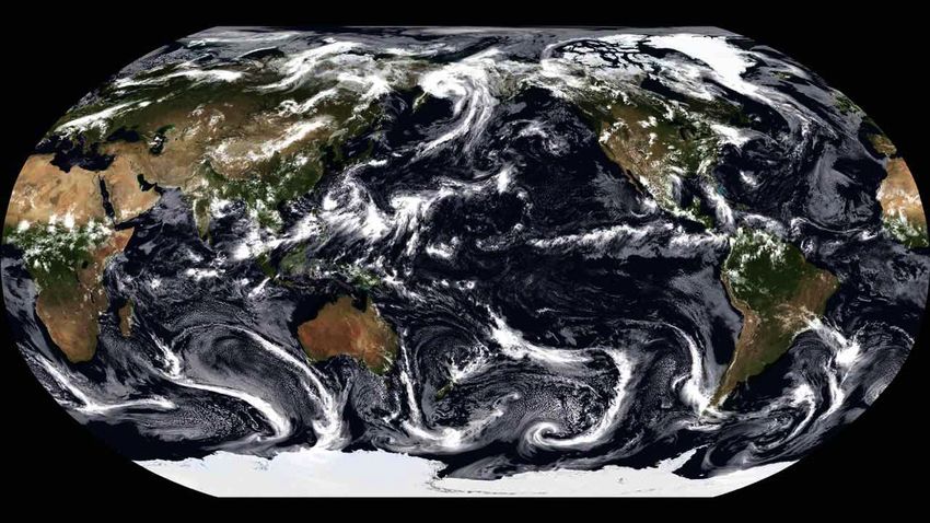
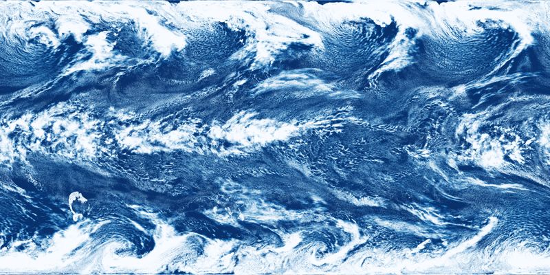
Can we apply same ML approach to GFDL’s 3 km FV3-GFS global atmospheric model?

 FV3-GFS DYAMOND run
 S.-J. Lin and Xi Chen, GFDL

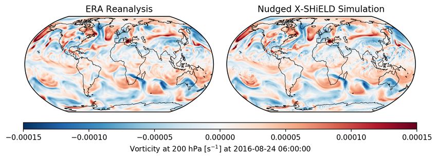
Training dataset: nudged 3 km SHiELD (modified
FV3-GFS)
• Training dataset: 40 d ‘nudged DYAMOND’ simulation on GAEA (1 Aug to 9 Sep 2016):
• Observed SSTs
• Light nudging ( = 1 day) of 3 km T/u/v/ps to ERA5 reanalysis keeps meteorology ‘data-
 aware’. Nudging tendencies are considered to be part of the learned physics
• Store atmospheric and land-surface restart fields coarse-grained to 25 km every 15 min

Improved diurnal cycle of precipitation over land

 3 km SHiELD

 200 km resoluCon
 GCM

CorrecBng model errors with machine learning

• Uncorrected coarse model:

​(​ ​ ↓ / )↓0 =​ ↓ + ​ ↓ ↑ , ​ ↓ =−​ ↓ ⋅∇​ ↓ 
• Coarse model can include no physics (​ ↓ ↑ = 0) or a subset of parameterized
 physical processes that help track the fine-grid model (e. g. turbulence, radiation,
 clouds, Cu parameterization).

• Machine-learn a state-dependent corrective source ∆​ ↓ for the coarse model:

 ​ (​ / )↓ =​(​ ​ ↓ / )↓0 +Δ​ ↓ =​ ↓ +​ ↓ ↑ +Δ​ ↓ 

• Apparent moistening: ​ ↓2 =​ ↓​ ↓ ↑ +Δ​ ↓​ ↓ 

Tendency difference method for computing
correcting source
 Coarsened state of fine-resoluCon model saved every 15 minutes.
 Fine-res tendencies computed from these snapshots.
 ​ ​ ↓ / 

 ​(​ ​ ↓ / )↓0

 Coarse-resoluCon model iniCalized from each CorrecCng source:
 coarsened high-resoluCon snapshot and run
 forward for 15 minutes, with a 1-minute Cmestep. Δ​ ↓ =​ ​ ↓ / − ​(​ ​ ↓ / )↓0

 Low-res tendencies computed from final minute.

Baseline model physics

We run ML on top of several configuraCons of the coarse-resoluCon model:
1. physics-on
 • All physical parameterizaCons on
 (land surface, boundary layer, convecCon, radiaCon, microphysics, gravity wave drag)
2. clouds-off
 • Deep and shallow convecCon schemes off
 • No microphysics
 • Use clear-sky radiaCon only
3. physics-off
 • Run only dynamical core

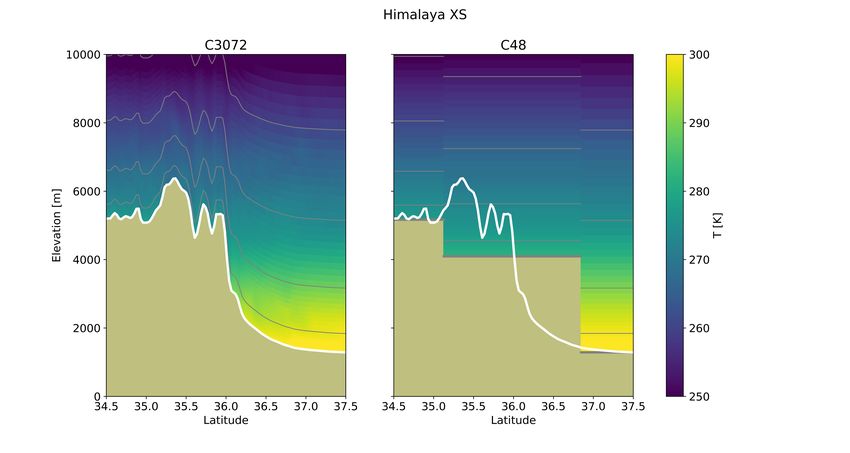
Conceptual issues over topography
Consider 3 km -> 200 km coarse-graining over the Himalayas

 • We coarse-grain to obtain
 verCcal profiles and apparent
 sources of T, q, etc.
 • 5 km relief within a coarse cell
 • Most fields are much more
 constant along a pressure
 surface than along a terrain-
 following model surface

 → Coarse-grain on pressure levels,
 not model levels

Machine learning: model training
Training set = 1.7M samples (130 iniCalizaCons x 13824 grid points)
Test set = 660K samples (48 iniCalizaCons x 13824 grid points)
Train/test data separated by split date to minimize correlated data across sets

 Random forest model

 • Ensemble of 13 decision tree es:mators, each
 with max depth of 13
 • Easier to run with stability in prognos:c
 simula:ons (rela:ve to neural nets)

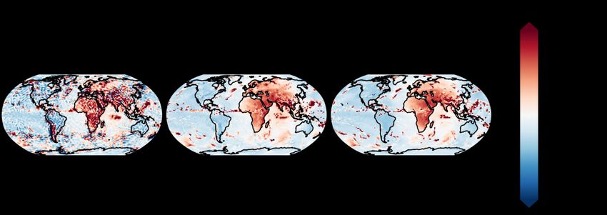
Machine learning: diagnostic skill
Column integrals of the ML-predicted verCcal profiles reproduce spaCal features of
net heaCng and precipitaCon, while also smoothing out noise from coarse-graining
and iniCalizaCon.

 Cme avg
 ML model predicCon Test data target

 [W/m2]
 Net ML-implied heaBng

 ML model predicCon Test data target

 - Cme avg
 [mm/d]
 Net ML-implied precipitaBon

 ML model trained with clouds-off
 configuraCon

2-day prognostic forecast of precipitation

3 km simulaCon averaged to 200 km FV3GFS with deep
hourly 25 km convecCon param replaced
 by ML

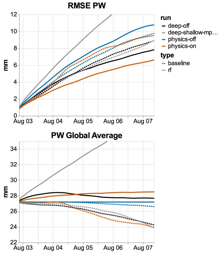
Weather forecast test
• 5-10 day ‘weather forecasts’ are an acknowledged test of
 global atmospheric model skill

• Goal is to match the evolution of the 3 km training model.

• Skill metric: root-mean-square error (RMSE) of map of column
 water vapor in 200 km model vs. coarsened 3 km model.
 Smaller is better.

• RMSE grows as coarse model diverges from training model.

• “Climate” skill metric: minimal global-mean drift over 5 days

• Currently, the best model configuration includes all
 conventional physics parameterizations and no ML.

• Most (not all) ML runs to date crash between 5 and 10 days

• …but it’s early days, and we are working to improve ML skill.

Alternative strategies for computing corrective
sources
 Snapshot of net column-heaCng in training dataset:

 Tendency difference Nudging coarse-model High-resoluBon physics budget
 method (noisy) towards the high-res informaCon + eddy flux
 convergence
 (like Yuval and O’Gorman 2020)

 TesCng these soon!

Conclusions and Outlook

• VCM has developed a unique cloud-based workflow for training a ML
 correction to a coarse-resolution climate model based on fine-resolution
 GSRM simulations.
• We have trained stable ML schemes that can make skillful global rainfall
 forecasts over land and ocean for 10 days or longer given specified SST.
• Tendency-difference method is flexible but is degraded by vertical velocity
 transients
• Promising new approaches to improve training data quality

Thank You!

hBps://vulcan.com/Our-Work/Climate/Climate-Modeling-aspx

FV3GFS and SHiELD1 global weather/climate models
• FV3GFS: Open-source global atmosphere model used by NOAA for operational weather forecasts
• FV3 dycore – Customized D-grid finite volume method on cubed sphere.
• Nonhydrostatic by default, 80 vertical levels used here.
• Specified time-varying sea-surface temperature used here
• Horizontal grid resolutions:
 • 3 km (C3072) No deep cumulus parameterization or gravity-wave drag
 • 13 km Used for NCEP’s current operational global weather forecasts
 • 25 km Finest grid currently practical for climate simulations of many decades
 • 200 km (C48) Typical coarse climate model grid – good for prototyping or millennial runs.
• Physical parameterizations:
 • Land surface and surface fluxes (NOAH)
 • Radiation (RRTMG)
 • Gravity-wave drag
 • Boundary-layer (including shallow clouds) and shallow Cu (Han-Bretherton, Han-Pan)
 • Cloud microphysics and subgrid variability (GFDL one-moment)
 • Deep cumulus convection (SAS)

1 GFDL’s SHiELD is FV3GFS with modest changes to cloud physics and advection and is not open-source.

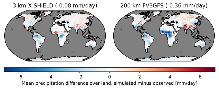
40 d mean precipitation bias over land: 3 km SHiELD vs.
200 km FV3GFS

 (GPCP)

 3 km rainfall bias much smaller over sub-Saharan Africa and Himalayas
 Diurnal cycle of precipitaCon over land is also greatly improved in SHiELD

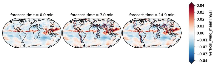
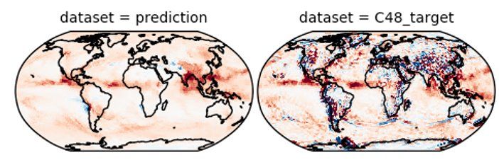
Despite careful efforts of pressure-level coarse-graining,
 vertical velocity noise remains over topography
 VerBcal velocity in upper troposphere (~250hPa)

 Averaged over 348 iniCalizaCon
 Cmes spanning training dataset.

 Fine resoluCon model
 coarsened to 200km
 resoluCon
These results are from clouds-off, but all physics configuraCons give comparable results