Modeling Microwave Waveguide Components: The Tuned Stub
←
→
Page content transcription
If your browser does not render page correctly, please read the page content below
Modeling Microwave Waveguide Components: The Tuned
Stub
Roger W. Pryor, Ph.D.1
1
  Pryor Knowledge Systems
*Corresponding author: 4918 Malibu Drive, Bloomfield Hills, MI, 48302-2253, rwpryor@pksez1.com

Abstract: The waveguide device modeled here           to perform a two-port S-parameter analysis of a
specifically demonstrates the exploration of a        Three Stub Tuner in the range of 2.2 to 3.3
small, but very important, subset of components       GHz.
of the family of microwave hardware devices               One of the primary advantages of using
designed to facilitate the optimized transfer of      COMSOL Multiphysics software is the inherent
power from the generating source to the               capability of the modeler to modify or create, as
consuming load. Each of those components is           needed, suitable equations for insertion into the
called, in electronics terminology, a Tuned           model for the calculation of the model
Stub.                                                 parameters or for the incorporation of data into
                                                      visualization plots.
    A stub is a length of transmission line or
waveguide that is connected to the active circuit         In the case of this 3D model, it was
at one end only. This paper models a                  necessary to add the equation for the calculation
rectangular waveguide with three adjustable           of the Voltage Standing Wave Ratio (VSWR).
stubs distributed along the upper surface of the      The VSWR is a measure of the power transfer
waveguide. The waveguide stubs are hollow, as         match and indirectly of the potential signal
is the waveguide, and they are each                   dispersion and/or distortion.
electromagnetically connected to the inner
cavity, at right angles to the central axis of the    2. Designing the Three-Stub Tuner
waveguide via an aperture in the wall of the          Model
waveguide. In this case, three (3) stubs have
been added along the length of the waveguide              A stub {1} is a length of transmission line
to optimize the tuning performance.                   or waveguide that is connected to the active
                                                      circuit at one end only. The stub can be either
Keywords: waveguide, microwave, tuned-stub,           open-circuited or short-circuited at the
VSWR, power-transfer.                                 unconnected end. In this case, the stubs are
                                                      short-circuited at the unconnected end and there
1. Introduction                                       are three stubs distributed along the length of
                                                      the waveguide segment.
    Microwave signals need to be clear and
undistorted to ensure accurate information
transfer. The primary function of many
waveguide systems is to convey a complex,
broad       power       range,     wave-based,
electromagnetic signal from the generating or
receiving source to the consuming or input load
with a minimum of signal dissipation and/or
distortion. Since waveguides have great
technological importance and application
diversity, they are designed and manufactured
in a large range of wave-length-specific,
application-dictated,    shapes,  sizes,    and
configurations.
                                                                   Figure 1. Three Stub Tuner.
   In this paper, the COMSOL Multiphysics
RF Module software (version 4.3) is employed

             Excerpt from the Proceedings of the 2012 COMSOL Conference in Boston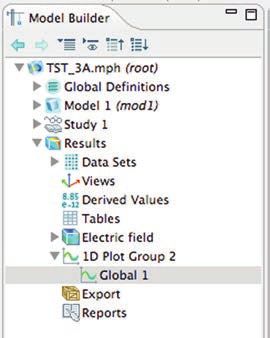
Figure 1 shows a diagram of a section of analysis of a Three Stub Tuner in the range of
rectangular waveguide with three adjustable 2.2 to 3.3 GHz, the electromagnetic field results
stubs distributed along the upper surface of the of which are shown in Figure 2.
waveguide. The Figure 1 configuration is the
basis of the model in this paper. Each of the S-parameter analysis {2, 3} is one of a
waveguide stubs is a hollow, rectangular cavity, number of different complex methodologies
in a similar manner to the primary waveguide. that can be used to analyze the properties of
Each stub is orthogonally mechanically circuits at RF and microwave frequencies. The
coupled, as shown in Figure 1, to the primary S-parameter methodology employs matched-
inner waveguide cavity, via an aperture in the load terminations, rather than short-circuit or
top-wall of the waveguide. These stub- open-circuit terminations. The use of S-
connected apertures in the top-wall electro- parameter methodology {4} lends itself well for
magnetically couple the stubs to the main use in the processing of complex matrices and
waveguide cavity. complex matrix calculations.
The stubs are short-circuited at the The Model Builder Tree of the completed
unconnected end and open-circuited at the COMSOL Multiphysics model is shown in
waveguide-connected end. Rotating the blue Figure 3.
knob shown in Figure 1, at the top of each stub,
varies the electrical and the mechanical length
of each stub. Stub tuners may be designed to
have any number of stubs (1, 2, 3, etc.).
Figure 3. Three Stub Tuner Model Builder Tree.
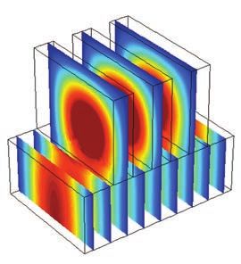
Figure 2. Three Stub Tuner Calculated Field- 3.1 Building the Three Stub Tuner Model
Distribution Solution.
You can start building the Three Stub Tuner
As can be seen in the calculated field- Model on the COMSOL Multiphysics Desktop
distribution solution displayed in Figure 2, three in Model Builder by selecting 3D > Next >
(3) stubs have been appended along the length Radio Frequency > Electromagnetic Waves,
of the waveguide to strive for an optimized Frequency Domain (emw) > Add Physics >
performance of the final tuner design. The Next > Custom Studies > Empty Study >
construction details of this model are presented Finish. Figure 4 shows the initial Model Builder
and discussed in the body of this paper. Tree.
3. Modeling Using the RF Module in
COMSOL Multiphysics 4
In this paper, the RF Module of the
COMSOL Multiphysics software (version 4.3)
is employed to perform a two-port S-parameter
Excerpt from the Proceedings of the 2012 COMSOL Conference in Boston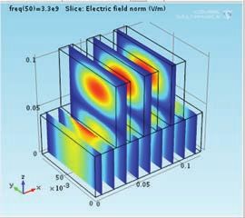
Click on Step 3: Frequency Domain, then go to
                                                   the Frequency Domain settings window and
                                                   Click on the Range Settings button. Enter the
                                                   parameters shown in Table 2.

                                                   3.2 The Three Stub Tuner Model Geometry

                                                       The Three Stub Tuner geometry comprises
                                                   the union of 4 rectangular prisms. The
                                                   configuration data, as defined in the Appendix
                                                   in Table 3, should be entered in the model, as
                                                   follows: Right-Click Global Definitions > select
                                                   Parameters and enter the data in the Parameters
          Figure 4. Three Stub Tuner Initial       edit window.
                Model Builder Tree
                                                       Build the Three Stub Tuner geometry as
    In the next set of steps, the 3D Three Stub    follows: Right-Click on Geometry 1 and select
Tuner model is configured to use Boundary          Block. Go to the Block 1 Settings window and
Mode Analysis {5}. The Boundary Mode               enter the first six (6) parameters in the Size and
Analysis sets up the parametric configuration      Shape and Position global data parameters edit
for the creation and analysis of Port 1 and Port   windows. Once entered, Click > Build Selected.
2.                                                 Create each additional Block using the same
                                                   methodology with the next new set of six (6)
    Right-Click on Study 1 in Model Builder        global data parameters.
and select Study Steps > Boundary Mode                 Once all four (4) blocks have been created,
Analysis. Configure the Step 1: Boundary           then you can Right-Click Geometry 1 and select
Analysis Settings as shown in the Appendix in      Boolean Operations > Union. Click Zoom
Table 1. Figure 5 shows the Settings for Step 1    Extents in the Graphics Toolbar. Then, Select
in place. Create and configure Step 2: Boundary    all four (4) of the domains and add them to the
Mode Analysis using the same methodology.          Union Selection window. Uncheck the Keep
Configure the Settings for Step 2, as shown in     interior boundaries checkbox. Click Build All.
Table 1.
                                                     The final configuration of the Three Stub
                                                   Tuner Model is as shown in Figure 6.

                                                        Figure 6. Three Stub Tuner Model Geometry
         Figure 5. Boundary Mode Analysis
                 Settings for Step 1                  The last parameter entry in Table 3 is the
                                                   value of the wall conductivity, which will be
   Right-Click on Study 1 in Model Builder         used in defining the wall material of the Three
and select Study Steps > Frequency Domain to       Stub Tuner walls and is used in calculating the
add Step 3. The Frequency Domain Settings are      wall losses of the tuner.
as shown in the Appendix in Table 2. First,

            Excerpt from the Proceedings of the 2012 COMSOL Conference in Boston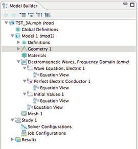
3.3 The Three Stub Tuner Model Materials              Next, Right-Click on the Electromagnetic
                                                   Waves, Frequency Domain (emw) Module and
   The Three Stub Tuner Model comprises two        Select Port from the pop-up window. Click on
materials: the domain = vacuum and the (wall)      Port 1.
boundaries = very thin conductive sheets (e.g.
Silver).                                               Select Boundary 1 in the Graphics window.
                                                   Add Boundary 1 to the Port Selection window
    Right-Click on Model Builder > Model 1 >       in the Settings Page. In Port > Port Properties,
Materials and then Select Material from the        Set the Type of port to Numeric and the Wave
pop-up window. Right-Click on Material 1 >         excitation at this port to On.
Select > Rename. Enter Vacuum as the name of
the material and Click OK.                            Now, Right-Click on the Electromagnetic
                                                   Waves, Frequency Domain (emw) Module and
   In the Material Selection edit window, add      Select Port from the pop-up window. Click on
Domain 1. In the Material > Material Contents      Port 2.
edit window enter the values of the properties
shown in Table 4.                                      Select Boundary 24 in the Graphics window.
                                                   Add Boundary 24 to the Port Selection window
    Right-Click on Model Builder > Model 1 >       in the Settings Page. In Port > Port Properties,
Materials and then Select Material from the        Set the Port name to 2, the Type of port to
pop-up window. Right-Click on Material 2 >         Numeric and the Wave excitation at this port to
Select > Rename. Enter Lossy Wall Material as      Off.
the name of the material and Click OK.
                                                   3.4 The Three Stub Tuner Model Mesh
                                                   Configuration
   In the Material Geometric Entity Selection
edit window, Select Boundary from the pull-            Right-Click Model Builder Mesh, Select
down list. Add Boundaries 2-23 to the Selection    Free Tetrahedral from the pop-up list. Click on
edit window.                                       Mesh 1 > Size. On the Size Settings page, in the
                                                   Element Size Parameters > Maximum element
   In the Material > Material Properties > Basic   size edit window, Enter 0.006.
Properties list, select and add the Basic
Properties shown in Table 5. In the In the
Material > Material Contents edit window,          3.4 The Three Stub Tuner Model
Enter the parameter values for each property as    Computation
shown in Table 5.
                                                      Right-Click on Study 1, Select Compute.
3.4 The Three Stub Tuner Model
Electromagnetic Waves, Frequency Domain
Configuration                                      4. The Three Stub Tuner Results

   To configure the Electromagnetic Waves,            The default plot is a Multislice plot with one
Frequency Domain (emw) Module, Right-Click         plot plane in each of the primary directions (x,
on the Electromagnetic Waves, Frequency            y, z). To create the plot shown in Figure 2,
Domain (emw) Module and Select Impedance           Right-Click on the Results > Electric field >
Boundary Condition from the pop-up window.         Multislice icon and Select Delete.

    Click on Impedance Boundary Condition 1.           Next, Right-Click on the Results > Electric
In the Graphics window, Select boundaries 2-23     field and Select Slice. Click on Slice 1. Go to
and add them to the Selection edit window in       the Slice Settings page and enter 9 in the Slice >
the Impedance Boundary Condition Settings          Plot > Plane Data > Planes edit window. Click
page.                                              Plot in the toolbar. The resultant plot is shown
                                                   in Figure 7.

            Excerpt from the Proceedings of the 2012 COMSOL Conference in Boston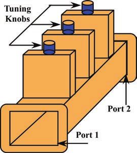
The VSWR plot is shown in Figure 8.

          Figure 7. Three Stub Tuner Model
                Electric Field Result                       Figure 8. Three Stub Tuner Model
                                                                       VSWR Plot
4.1 The Three Stub Tuner Model VSWR
Calculation                                        5. Conclusions
    The VSWR (Voltage Standing Wave Ratio)            A new model has been developed and
is defined mathematically as:                      presented for the Three Stub Tuner, a critical
                                                   microwave component. This model shows the
                           1+ S11                  electric field distribution and the VSWR. The
   1.           VSWR =                             VSWR graph shows that the Three Stub Tuner
                           1− S11                  has almost no power reflection in the range
                                                   from 2.4 GHz to 3.3 GHz.
Where S11 is the Port 1 scattering coefficient        This model demonstrates that the RF
and is calculated by the RF Module.                Module of COMSOL Multiphysics software
                                                   can be easily employed, when properly
   To plot the VSWR, Right-Click on Model          configured, to calculate microwave component
Builder > Results, Select 1D Plot Group from       power distribution and reflection analysis
the pop-up list. Next, Right-Click on 1D Plot      problems.
Group 2, Select Global from the pop-up list.
Click on Global.

   Enter, as the y-axis data Expression:

   2. (1 + abs(emw. S11)) / (1 − abs(emw. S11))

   Click > Plot in the Toolbar.

             Excerpt from the Proceedings of the 2012 COMSOL Conference in Boston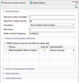
6. References                                    7. Appendix

1. http://en.wikipedia.org/wiki/                   Table 1: Boundary Mode Analysis Step Settings
          Stub_(electronics)
2. http://en.wikipedia.org/wiki/Scattering_           Parameter              Step 1         Step 2
          parameters                                  # of Modes                1              1
                                                   Search for Modes            50              50
3. COMSOL RF Module Users Guide, pp 42-48
                                                      Transform              out of       out of plane
4. COMSOL RF Module Users Guide, pp 43,                                       plane
waveguide_adapter model.                              Port name                 1              2
5. COMSOL RF Module Users Guide, pp 135-          Analysis frequency       2.45[GHz]      2.45[GHz}
136
6. COMSOL Multiphysics Users Guide, pp 78               Table 2: Frequency Domain Settings
7. COMSOL Multiphysics Users Guide, pp 580
                                                          Step                       Value
                                                          Start                       2.2e9
                                                          Step                      1.1e9/49
                                                          Stop                        3.3e9

                                                   Table 3: Three Stub Tuner Geometry Parameters

                                                   parameter             value           description
                                                     Wg_ht             43.18[mm]          Waveguide
                                                                                        inside height
                                                    Wg_dp              86.36[mm]          Waveguide
                                                                                         inside depth
                                                    Wg_wd             122.45[mm]          Waveguide
                                                                                         inside width
                                                     x0_cnr              0[mm]            x corner of
                                                                                          Waveguide
                                                     y0_cnr              0[mm]            y corner of
                                                                                          Waveguide
                                                     z0_cnr              0[mm]            z corner of
                                                                                          Waveguide
                                                    Stb1_ht            6.1224[cm]        Tuning stub
                                                                                            height
                                                    Stb1_dp            86.36[mm]         Tuning stub
                                                                                             width
                                                    Stb1_wd            1.5306[cm]        Tuning stub
                                                                                            length
                                                     x1_cnr           22.959[mm]       x corner of stub

                                                     y1_cnr              0[mm]         y corner of stub

                                                     z1_cnr            43.18[mm]       z corner of stub

                                                    Stb2_ht            6.1224[cm]        Tuning stub
                                                                                            height
                                                    Stb2_dp            86.36[mm]         Tuning stub
                                                                                            width
                                                    Stb2_wd            1.5306[cm]        Tuning stub
                                                                                            length
                                                     x2_cnr           53.571[mm]       x corner of stub

                                                     y2_cnr              0[mm]         y corner of stub

           Excerpt from the Proceedings of the 2012 COMSOL Conference in Boston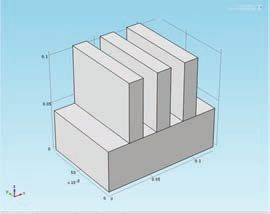
parameter           value             description
    z2_cnr          43.18[mm]         z corner of stub

   Stb3_ht          6.1224[cm]          Tuning stub
                                           height
   Stb3_dp          86.36[mm]           Tuning stub
                                           width
   Stb3_wd          1.5306[cm]          Tuning stub
                                           length
    x3_cnr         84.184[mm]         x corner of stub

    y3_cnr            0[mm]           y corner of stub

    z3_cnr          43.18[mm]         z corner of stub

  sigma_wall        6.3e7[S/m]            Wall cond.

Table 4: Three Stub Tuner Material: Vacuum

                  Vacuum
 Property          Name          Value          Unit
  relative        epsilonr         1             1
permittivity
  relative          mur               1           1
permeability
 electrical        sigma         1.0e-9         S/m
conductivity

Table 5: Three Stub Tuner Material:
          Lossy Wall Material

                   Wall
 Property          Name          Value          Unit
  relative        epsilonr         1             1
permittivity
  relative          mur               1           1
permeability
 electrical        sigma      sigma_wall         S/m
conductivity

               Excerpt from the Proceedings of the 2012 COMSOL Conference in Boston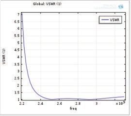
You can also read