Market Transparency and Consumer Search - Evidence from the German Retail Gasoline Market - Simon Martin September 2020 - HHU
←
→
Page content transcription
If your browser does not render page correctly, please read the page content below

NO 350

Market Transparency and Consumer Search –
Evidence from the German
Retail Gasoline Market
Simon Martin

September 2020

IMPRINT

D IC E D I SCU SSI ON PAP E R

Published by:
Heinrich-Heine-University Düsseldorf,
Düsseldorf Institute for Competition Economics (DICE),
Universitätsstraße 1, 40225 Düsseldorf, Germany
www.dice.hhu.de

Editor:
Prof. Dr. Hans-Theo Normann
Düsseldorf Institute for Competition Economics (DICE)
Tel +49 (0) 211-81-15125, E-Mail normann@dice.hhu.de

All rights reserved. Düsseldorf, Germany 2020.

ISSN 2190-9938 (online) / ISBN 978-3-86304-349-0

The working papers published in the series constitute work in
progress circulated to stimulate discussion and critical comments.
Views expressed represent exclusively the authors’ own opinions
and do not necessarily reflect those of the editor.
Market Transparency and Consumer Search -
   Evidence from the German Retail Gasoline Market

                                        Simon Martin*

                                       September 2020

                                             Abstract

          We study a novel trade-off in market transparency regulation by estimating a
      structural model of the German retail gasoline market. Transparent environments
      enable easy price comparisons and match findings. Restricting transparency such
      that only the cheapest offers are shown induces firms to compete for attention,
      but matching is inefficient. We find that there is an inverse u-shaped relationship
      between consumer welfare and market transparency. Consumer welfare is maximal
      when only the first 20% of prices are shown, which decreases consumer expenditures
      by 1.2%. Our framework allows estimating games of incomplete information with
      very lax data requirement.

      Keywords: market transparency, consumer search, awareness, consideration sets,
      retail gasoline prices

      JEL Codes: D22, D43, D83, L13, L50

  * Düsseldorf   Institute for Competition Economics (DICE). Email:      simon.martin@dice.hhu.de.
I would like to thank Daniel Garcı́a, Alessandro Gavazza, David Genesove, Marc Goñi, Bernhard Kas-
berger, Maarten Janssen, John Morgan, Karl Schlag, Philipp Schmidt-Dengler, Frank Verboven, Matthijs
Wildenbeest, and participants in seminars at the VGSE, University of Mannheim, NHH Bergen, Copen-
hagen Business School, University of Copenhagen, Universidad Carlos III de Madrid, DICE, the QED
Jamboree 2018 (Alicante), the ZEW Summerworkshop 2018 (Mannheim), EARIE 2018 (Athens), and
EEA-ESEM 2019 (Manchester) for useful comments and suggestions. Funding from the Austrian Science
Fund (P 30922) is gratefully acknowledged.

                                                 1
1     Introduction
Regulating market transparency is an important policy issue in various jurisdic-
tions. The main objective of this regulation is to provide consumers with better
information and thereby tighten competition. Several countries have introduced
government-operated comparison websites in the last decade, e.g., for financial prod-
ucts, energy markets, and retail gasoline markets. Simplified comparisons should
reduce information frictions as a source of market power and lead to lower prices
(Varian, 1980, Stahl, 1989, Wolinsky, 1986). However, firms may also find it easier
to monitor their competitors, making the market more prone to tacit collusion and
thus leading to higher prices (Kühn and Vives, 1995, Ivaldi et al., 2003).
    These considerations suggest that full transparency is consumer welfare optimal
as long as it primarily affects consumers. In this paper, we provide both theoretical
and empirical evidence that this intuition is wrong. It is true that the “comparison
effect” makes consumers worse off since they can compare only a smaller set of
options. Yet one also needs to take into account the equilibrium response of firms.
Restricting transparency by only informing consumers about cheap offers induces
firms to compete fiercely for precious spots in the consumers’ consideration set.
We call this the “attention effect.” When the attention effect is sufficiently strong,
prices may be lower in a restricted transparency regime.
    In addition, there is also a “matching effect” when products are horizontally and
vertically differentiated, e.g., because of travel costs. Consumers may be worse off
in an environment that induces low prices at the expense of low match quality.
    This paper complements the literature on market transparency (Luco, 2019,
Dewenter et al., 2016, Ater and Rigbi, 2017, Rossi and Chintagunta, 2016) by de-
scribing and quantifying the attention and matching effect. We also make a method-
ological contribution by developing a framework that allows estimating games of
incomplete information using only publicly available data.
    Our aim is to understand the overall effect limiting transparency has on prices
and consumer welfare. In particular, we are interested in whether the benefits due
to the attention effect outweigh the downside owing to the matching effect. We
set up a novel model that includes both effects and take it to the data. Retail
gasoline markets are an ideal environment for studying these forces since product
differentiation can be neatly modelled and estimated. The rich history of prices
is readily available. Specifically, we provide an answer to the following question:

                                          2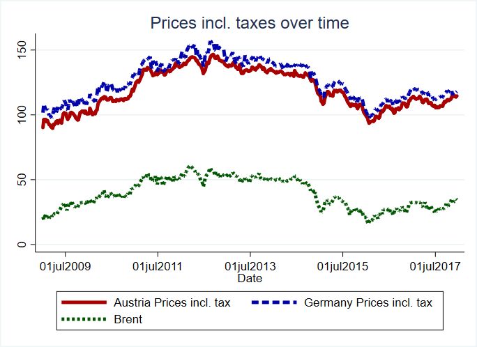
What is the effect on prices and match quality should Germany change the market
transparency regulation? The economic forces revealed in this paper also apply to
numerous other markets and industries with information frictions.
   In order to address these questions, we develop and estimate a structural model
of the German retail gasoline market. Both the attention and the matching effect
arise naturally in our environment. Given estimated model parameters, we conduct
counterfactual policy simulations by computing equilibrium prices under different
transparency regimes.
   Our main finding is that there is an inverse u-shaped relationship between market
transparency and consumer welfare. Consumer welfare is maximal at intermediate
levels of market transparency. The exact level of course depends on the environ-
ment, but for the German retail gasoline market, showing only 20% of stations is
optimal. In that case, quantity-weighted prices decrease by 1.2% and consumer
welfare increases by 3.9% of firms’ current margins. Although prices fall further
when less then 20% of stations are shown, consumer surplus decreases due to inef-
ficient matching. Online consumers are only informed about low-quality stations,
and high-quality stations price exclusively to their loyal customer segment, making
consumers worse off. Hence, the relationship between consumer welfare and market
transparency is non-monotonic.
   Our model incorporates key features of markets with information frictions. “On-
line consumers” become informed about stations and prices online. The regulator
chooses the “transparency regime,” i.e., a cutoff point ρ such that only the ρ% cheap-
est prices are displayed online. Thus, consideration sets depend endogeneously on
prices, giving rise to both the attention and matching effect. Since December 2013,
German gasoline stations have been obliged by law to transmit prices to a central
database operated by the Market Transparency Unit (MTU). Various websites ac-
cess the MTU’s database and provide consumers with real-time price information.
Our model allows us to quantify both the attention and the matching effect and,
given estimated parameter values, we conduct counterfactual policy simulations.
   These counterfactual scenarios are motivated by observed variation in the trans-
parency regulations of retail gasoline markets across countries. For instance, Ger-
many and France provide websites that are fully transparent. Consumers can learn
all the prices they might possibly be interested in. Conversely, Austria’s website
provides only restricted transparency: For any given address, only the first half of

                                          3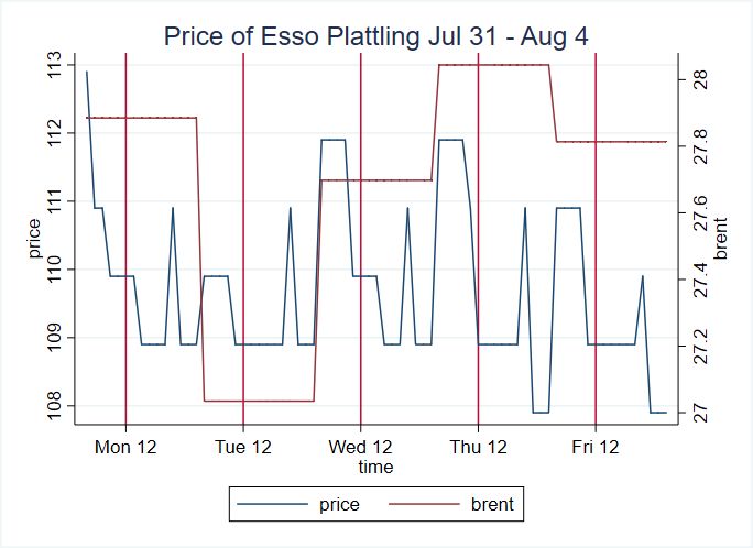
the nearby prices are shown. We explain the reason for this restriction in detail
below.
   We find that the attention effect is very strong. In the first counterfactual
scenario we simulate Germany adopting the Austrian regime of showing only the
cheapest 50% of stations. Quantity-weighted prices decrease by 0.6% and average
prices decrease by 0.5%. Decomposing the total effect, we find that the compari-
son effect increases average prices by 1.1%. Since the attention effect is stronger,
decreasing average prices by 1.6%, the net effect on prices is negative.
   The undesired matching effect of restricting transparency stems from low-quality
firms with lower marginal costs. These are more inclined, on average, to charge low
prices in order to appear on the restricted price list and hence in the consumers’
consideration set. Thus, the price list more often contains low quality stations,
making consumers fuel their car at cheaper stations with fewer amenities and pos-
sibly further away from them. This partially mitigates the positive effect on con-
sumer surplus through lower prices. The increase in consumer surplus is exclusively
through uninformed consumers who benefit from lower prices. Online consumers, on
the contrary, are actually worse off under restricted transparency due to inefficient
matching.
   Our paper contributes to the literature by overcoming both theoretical and em-
pirical challenges in novel ways. In our model, intertemporal equilibrium price dis-
persion arises due to private-information marginal cost shocks, resulting in a game
of incomplete information. This approach eliminates Bertrand-type undercutting
motives and gives rise to pure strategy equilibria. Our environment allows for a
close link between theory and reality with respect to the representation of consider-
ation sets. Online consumers are informed exactly about all the stations displayed
online. We thereby avoid the necessity of introducing additional noise in the infor-
mation acquisition and hence an additional ‘information elasticity’ parameter to be
estimated (Sovinsky Goeree, 2008, Honka et al., 2017, Dinerstein et al., 2018).
   Empirically, a major challenge in our environment is the unavailability of demand-
side data or market shares. Therefore, standard approaches like Berry et al. (1995)
that simultaneously estimate supply- and demand-side parameters and implied elas-
ticities are not feasible. Our approach is based on Thomadsen (2005). We exploit
the fact that different brands are observed repeatedly in different market configu-
rations. For instance, a Shell and a BP station may compete with each other in

                                         4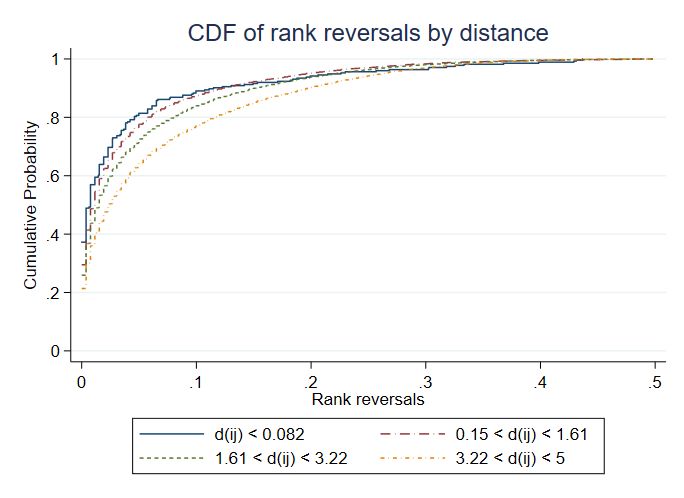
two different markets, where the distances between them differ. We assume that
demand is deterministic given prices and hence the only source of noise stems from
marginal cost shocks. Then we can use the firms’ first-order conditions to estimate
the structural parameters due to the non-linearities in optimal pricing with respect
to distance. Under a similar argument, variation in the number of stations per
market and variation in the input prices in a given market over time independently
identify the parameters of interest. We combine all these sources of variation and
additionally employ macro moments to enhance efficiency.
   This estimation approach requires detailed information about consumers’ loca-
tions in order to proxy for demand characteristics. We exploit building information
publicly available on Open Street Maps to construct an estimate of population den-
sity in 1x1km large cells. Distances to gas stations vary across cells, allowing for
very rich substitution patterns. Alternative approaches proposed in the literature
are based on consumers’ commuting patterns (Houde, 2012, Pennerstorfer et al.,
2020), which require highly detailed commuting data that is rarely available on a
large scale.
   Similar to approaches used in the auctions literature (Guerre et al., 2000, Athey
and Haile, 2002, 2007), we apply a two-stage estimation routine. In the first stage,
we fit the equilibrium price distribution for each station, conditional on the oil price.
These first-stage estimates are then used as equilibrium beliefs about competitors’
prices in the second stage. Finally, we back out the implied marginal cost shock
from the firms’ first-order conditions, given a parameter vector, and proceed with
a GMM estimation. Since the equilibrium of our incomplete information game is
somewhat involved and requires iteratively solving a set of integral equations, full
information approaches are essentially unfeasible. Our two-step approach eliminates
the computational burden of solving integral equations in each estimation step.
   The Austrian regulator enacted a restricted transparency regime due to concerns
of tacit collusion in a dynamic setting (Ivaldi et al., 2003, Albæk et al., 1997, Schultz,
2005, Petrikaitė, 2016). Nevertheless, we are convinced that considering a static set-
ting is appropriate in our environment. The retail gasoline market is already under
the close scrutiny of competition authorities in several OECD countries, includ-
ing Austria (Bundeswettbewerbsbehörde, 2011) and Germany (Bundeskartellamt,
2011, Bundesministerium für Wirtschaft und Energie, 2018). Hence, even if more
transparency could lead to more collusion and thus higher prices in theory, it seems

                                            5
very unlikely that this would be the case in practice. Additionally, even if average
expected prices increased, this still need not be detrimental for consumer welfare;
what we actually should be concerned about is the average price that consumers
actually pay, and how far they have to drive in order to make a purchase. Thus,
instead of explicitly modelling a dynamic environment, we estimate the static model
and provide convincing evidence that this model adequately captures key market
characteristics. Finally, we provide compelling evidence that reducing transparency
is in the consumers’ interest, even if it affects only the consumer side. If there is an
additional response on the firms’ side, the case for reducing transparency becomes
even stronger.
We proceed as follows. In the next subsection, we relate our paper to other ex-
isting literature. Section 2 provides an overview of the industry background and the
data, as well as the data collection process and descriptive evidence. The model is
developed and described in Section 3. The estimation and identification strategy as
well as parameter estimates are presented in Section 4. We show results from coun-
terfactual policy analysis and several robustness checks in Section 5, and conclude
in Section 6.
1.1 Related literature
Our paper relates to various strands of the literature. Government-mandated trans-
parency initiatives have recently triggered several empirical papers (Luco, 2019,
Dewenter et al., 2016, Ater and Rigbi, 2017, Rossi and Chintagunta, 2016, Mon-
tag and Winter, 2020). These papers typically conduct a difference-in-differences
analysis comparing price levels before and after the introduction of a transparency
website, which allows considering the two extremes of the spectrum of either no
transparency versus full transparency. As our results show, intermediate levels of
transparency may actually be optimal from a consumer surplus perspective. Our
structural estimates also reveal important insights on the underlying channels and
allow additional counterfactual simulations.
There is a vast literature on retail gasoline markets. Eckert (2013) provides a
comprehensive overview. Besides Luco (2019) and Rossi and Chintagunta (2016),
Nishida and Remer (2018) is close to this paper. Nishida and Remer (2018) estimate
the consumers’ search cost distribution for geographically isolated markets. They
show that, theoretically, policies that decrease both the mean and variance of the
6search cost distribution in a particular way may lead to higher prices. Measuring
how exactly transparency initiatives alter the search cost distribution is almost im-
possible. In our model information acquisition reflects exactly how price comparison
websites typically operate: Consumers are more likely to be informed about lower
prices. Firms in Nishida and Remer (2018) are vertically differentiated. We also
allow for horizontal differentiation and thus the matching and the attention effect
arise.1,2
In the literature to estimate search costs, it is common to exploit the indiffer-
ence condition of firms in a mixed-strategy equilibrium. This enables estimations
when market shares are unavailable (Hong and Shum, 2006, Moraga-González and
Wildenbeest, 2008). Wildenbeest (2011) extends this setup to a model of vertical
differentiation. This approach is not applicable to our setting where stations are also
horizontally differentiated due to their spatial location. Since in our setting firms
play an equilibrium in pure strategies, estimation based on indifference conditions
in mixed-strategy equilibria is not feasible.
The theoretical literature on information frictions is very broad and has become
increasingly relevant recently due to the rise of the Internet. Also in our model some
consumers are not informed, whereas others have the possibility of getting informed
through a central website that controls the flow of information. An important
difference is that in many of these models firms play mixed strategy equilibria
(Varian, 1980, Burdett and Judd, 1983) whereas in our model there are private-
information marginal cost shocks and firms play pure strategies given their cost
shock. Endogenous awareness sets are already considered, for example, in Butters
(1977), Sovinsky Goeree (2008), Honka et al. (2017), and Moraga-González et al.
1
Other re-occurring themes in the literature on gasoline markets, not specifically discussed here,
include asymmetric pass-through of input-cost shocks (Borenstein and Shepard, 1996, Borenstein et al.,
1997, Chandra and Tappata, 2011), Edgeworth cycles (Noel, 2007a,b, Wang, 2009, Eibelshäuser and
Wilhelm, 2017), regulation of frequency of price adjustment (Obradovits, 2014, Dewenter and Heimeshoff,
2012) and consumer learning about common input prices (Dana, 1994, Janssen et al., 2011). We are mostly
interested in price levels in this paper. In order to purge out the possible confounding effects of intra-day
pricing dynamics, we only consider prices at 5pm every day. The issue of learning does not arise in our
setting because consumers only consider stations whose price quote they have already obtained online.
2
There are also several empirical papers specifically about the German market (Haucap et al., 2016,
2017, Dewenter and Heimeshoff, 2012, Dewenter et al., 2016, Montag and Winter, 2020, Horvath, 2019)
and the Austrian retail gasoline market (Pennerstorfer and Weiss, 2013, Pennerstorfer et al., 2020). Since
the scope of these papers is very different to ours we do not discuss them in detail here.
7(2018). In these models awareness typically stems from the explicit advertising
expenditures of firms. In our model, the sole means through which firms get the
chance to advertise their prices are with the prices themselves: The probability
of making a consumer aware of their product depends wholly on prices, since the
government website ranks cheaper products higher. Finally, there are several recent
approaches to estimate heterogeneity in consideration sets across consumers (Heiss
et al., 2016, Abaluck and Adams, 2020, Barseghyan et al., 2020). In our model all
consumers who visit the website have the same consideration set.
Online price comparison websites have also strongly influenced the literature on
prominence and ordered search (Armstrong et al., 2009, Armstrong and Zhou, 2011,
Armstrong, 2017). Our theoretical result, that prices decrease as firms compete for
prominence (attention) through prices, is reminiscent of the main results in Arm-
strong and Zhou (2011). We additionally introduce the matching effect and explain
why it causes consumer welfare to be non-monotonic in transparency. Although con-
ceptually different, our finding that higher transparency may lead to higher or lower
prices is reminiscent of the ambiguous comparative statics in prices with respect to
search costs in Moraga-González et al. (2017) and Moraga-González et al. (2020).
Since we additionally allow for vertical differentiation and endogeneous prominence,
we provide additional insights in terms of consumer welfare.
Dinerstein et al. (2018) consider the role of platform design in online markets
and show that putting more weight on the price when displaying search results
intensifies competition. When products are sufficiently differentiated, this comes
at the expense of inefficient matching. This is similar to our finding that tougher
competition for a spot in the consumers’ consideration set may lead to lower prices
relative to full transparency, but worse matching. A key difference is that Dinerstein
et al. (2018) show that giving different information to consumers may be beneficial
for them; whereas we show that giving consumers even less information may be ben-
eficial for them. Dinerstein et al. (2018) consider online markets, whereas we show
the relevance of market transparency initiatives in offline markets. Additionally,
we establish a direct link between actually observed rankings and the consumers’
consideration set.
82 Industry background and data
In this section, we explain the industry background as well as relevant market
features. We show that there are persistent price differences as well as intertempo-
ral price dispersion, motivating our model with private-information marginal cost
shocks and both horizontal and vertical differentiation.
2.1 Market description and transparency regulation
In the German retail gasoline market, there are five major brands that operate
across the entire country and are strongly vertically integrated. Following Bun-
deskartellamt (2011), these are referred to as oligopoly players (Aral (BP), Shell,
Total, Esso, and Jet). The market leader Aral has a market share of around 16%
across Germany (according to the number of stations in 2017).3 The combined
market share of the five oligopoly brands is 51%. In line with the definition used by
Haucap et al. (2017), we additionally distinguish between ‘integrated’ brands (Orlen
(Star), Agip, HEM and OMV; combined market share 12%). All other brands are
referred to as ‘others.’
Retail gasoline stations in Germany are obliged to transmit prices to a central
database operated by the Market Transparency Unit (MTU, German Markttrans-
parenzstelle für Kraftsstoffe MTS-K), a subunit of the German competition author-
ity (Bundeskartellamt). This regulation was enacted in December 2013. Contrary
to the Austrian model where the regulatory body also operates the website to in-
form consumers, in Germany the MTU only operates the database. Information to
consumers is provided through privately operated websites and mobile apps, which
are given access to the MTU’s central database. There are 62 officially registered
websites and mobile apps.4 Gasoline stations in Germany are entirely unconstrained
in their price setting; in particular, they may increase their prices arbitrarily often
on any given day. A screenshot of one German price information provider (ADAC)
is shown in Figure 1. All stations and prices close to the stated address are shown.
On the Austrian price comparison website, only the cheapest stations are shown
(see Figure 2 for a screenshot of the market around Vienna, Austria).
Our analysis is based on the entire history of prices set in 2017, provided by the
3
https://www.mwv.de/statistiken/tankstellenbestand/
4
https://www.bundeskartellamt.de/EN/Economicsectors/MineralOil/MTU-Fuels/mtufuels node.
html, accessed June 2018.
9German website Tankerkönig,5 which in turn uses prices published by the German
MTU.
In addition to prices and rankings, we also observe the brand and various char-
acteristics for each station. We complement the dataset with additional regional
information on the population density from the German Federal Institute for Re-
search on Building, Urban Affairs and Spatial Development (BBSR).6 We proxy for
input prices using the Brent Crude Oil Price published by the US Energy Informa-
tion Administration7 and calculate the price in Euro cents per liter based on the
exchange rate published by the ECB (Janssen et al., 2011).8 Website usage statistics
are based on figures from the German Audit Bureau of Circulation (IVW).9 Total
gasoline and diesel consumption data were obtained from the Federal Office for
Economic Affairs and Export Control.10 Finally, we use building and road network
information publicly available from Open Street Maps.
We delineate markets based on municipality boundaries because it allows for
clean allocations and guarantees non-overlapping of markets, which is a key draw-
back of markets defined by circles around stations (Pennerstorfer et al., 2020).
Considering geographically isolated markets (Nishida and Remer, 2018) also avoids
overlapping markets, but is still somewhat arbitrary and may eliminate otherwise
relevant markets. We focus on municipalities with at least three stations and at most
315 1x1km large grid cells since we believe that in these markets our key considera-
tion of how market transparency shapes consumer choice plays the biggest role. In
very small markets, information acquisition online is less relevant to start with. In
larger cities there may be several additional forces at play that we may not be able
to address in a satisfactory manner. We thus omit these very large municipalities
altogether. Robustness checks are shown in Section 5.1. Since gasoline stations on
the highway are considered as a separate market by the German Bundeskartellamt,
we also omit them. In our sample there are 8,979 gasoline stations in 1,479 markets.
Table 1 gives an overview of the station characteristics.
5
http://tankerkoenig.de/
6
http://www.inkar.de/
7
https://www.eia.gov/dnav/pet/pet pri spt s1 d.htm
8
http://sdw.ecb.europa.eu/quickview.do?SERIES KEY=120.EXR.D.USD.EUR.SP00.A
9
http://ausweisung.ivw-online.de/
10
http://www.bafa.de/DE/Energie/Rohstoffe/Mineraloelstatistik/mineraloel$ $node.html
102.2 Intertemporal and cross-sectional price dispersion
Two key features of the German retail gasoline market are worth mentioning. First,
there are persistent price differences across stations and regions (see Table 1). Sec-
ond, both prices and the price ranking of stations vary over time. If consumers
knew which station was currently the cheapest, they might shop accordingly. In
our sample, the average number of daily price adjustments per station is 4.9 on
weekdays.
Intra-day price variation may result from systematic demand variation through-
out the day, e.g., morning and evening commuting patterns. In order to eliminate
these concerns, we restrict consideration to 5pm on weekdays, where most con-
sumers fuel their cars (Montag and Winter, 2020). Figure 3 shows the distribution
of the standard deviations of ranking across stations, which is very volatile. As an
example, figures 4 and 5 show the price and the price ranking, respectively, of the
Esso station in Plattling, Bavaria, over the first week of August 2017. The red ver-
tical bars denote noon on each of these days. Prices and rankings are very volatile
during the day and fluctuate much more than the oil price. One reason explaining
these fluctuations may be deterministic traffic flows during the day. Figure 6 shows
the ranking of the Esso station in Plattling, daily at 8am, which also fluctuates quite
heavily. Since traffic flows should be the same at the same time during weekdays,
they cannot explain the observed volatility.
The observed volatility in rankings is consistent both with firms playing mixed
strategies as well as with station-specific shocks that induce price changes. Chandra
and Tappata (2011) develop a test for mixed strategies and find clear support for it
in their data. They investigate rankings at the station-pair level. Stations pairs are
either “at the same corner” (which they define as being less than 270 feet away, i.e.,
0.082km, apart from each other) or not. Since information frictions should not be
present for stations at the same corner, differences in prices for those stations should
be driven exclusively by systematic differences. If stations at the corner change the
relative price rankings less frequently, this can be interpreted as a price setting that
is consistent with mixed strategies.
We implement the test of Chandra and Tappata (2011) and apply it to our
data. Figure 7 shows the CDF of rank reversals by distance as in Chandra and
Tappata (2011, Figure 7; see appendix for details). Table 2 shows coefficients from
regressing the dependent variable on an indicator for whether a station pair is on the
11same corner or not (Chandra and Tappata, 2011, Table 6). In contrast to Chandra
and Tappata, we do not find evidence that station pairs on the same corner are
systematically different from other station pairs. Fluctuations in rankings resulting
from shocks to marginal costs appear to be a better explanation for our data.
2.3 Descriptive evidence
We are interested in the effect of transparency regulation on prices. Currently,
Germany provides full transparency, whereas transparency in Austria is restricted.
Time series of the weekly average prices for Germany and Austria including and
excluding taxes are shown in Figure 8, respectively. These figures are based on the
Weekly Oil Bulletin published by the European Commission.11 Gross prices for
diesel are much lower in Austria (mean 119.0 CPL) than in Germany (126.0 CPL).
These differences are partially due to different tax rates. Excise duties on diesel are
currently 39.7 CPL (plus 20% Value Added Tax) in Austria and 47.04 CPL (plus
19% VAT) in Germany. In both countries, VAT is levied on the price including
the excise tax.12 Even accounting for different tax rates, net prices in Austria are
still lower (58.1 CPL vs. 58.8 CPL). We interpret these differences as evidence
in favor of restricted transparency. We cannot, however, claim causality based on
these numbers. Systematic price differences between countries might arise due to
several other reasons, e.g., regulation of price adjustment patterns (Obradovits,
2014) or other institutional patterns. Therefore, we cannot compare prices between
countries, but need to consider the effects in isolation within a particular country.
Thus, we next consider the main determinants of gasoline prices in Germany.
We present results from reduced-form regressions with prices per station as depen-
dent variable in Table 3. Naturally, the oil price (brent) is a key driver of price
setting. Oligopoly and integrated brands charge substantially higher prices than
other brands. Stations on the highway are even more expensive, lending support to
the claim that they form a separate market Bundeskartellamt (2011). The compet-
itive and spatial environment also play key roles. Prices decrease in the number of
stations. A prominent location close to consumers (distance-weighted population)
makes a gas station relatively more attractive and allows it to charge higher prices.
11
https://ec.europa.eu/energy/en/data-analysis/weekly-oil-bulletin
12
https://www.bundesfinanzministerium.de/Content/DE/Standardartikel/Service/Einfach erklaert/
2018-01-11-grundlagen-benzinpreis.html
12These results indicate that there is some relationship between prices, consumer
locations, and firm locations. In order to isolate the supply- and demand-side char-
acteristics, we develop and estimate a structural model in the following sections.
2.4 Consumer locations
Consumer locations and the distance to stations are among the determinants gov-
erning consumer demand from a respective gasoline station. We do not observe the
exact location, commuting patterns, etc., for each consumer at each point in time.
We proxy for consumer locations by assigning them to 1x1km large cells, based on
buildings information. Thomadsen (2005) uses census track data, which is readily
available for small census blocks in the US. An advantage of our approach over
methods considering only reported place of residence is that it takes into account
also likely work locations. Spatially matching almost 32m buildings to almost 1m
grid cells is a computationally heavy task that we accomplish using ArcGIS software
and the ArcPy Python plugin.
Our starting point is population data per municipality obtained from the German
Federal Institute for Research on Building, Urban Affairs and Spatial Development
(BBSR). For an illustration of our approach, consider the municipality Plattling,
Bavaria, shown in Figure 9. We obtain buildings data freely available from Open
Street Maps. The buildings in Plattling are shown in Figure 10. We assign the
municipality’s population to buildings proportional to the building ground area.
Since we cannot identify either the building height or the building type, we assume
that the building height within a municipality is uniform. We then project an
artificial fishnet over the entire area, creating 1x1km large cells (see Figure 11).
Finally, we calculate the sum of the proportional population per building in each
of these cells. The representative consumer per cell, used for distance calculations,
resides in the centroid of the cell.
3 Model
In light of the findings of the previous section, we present a model reflecting key fea-
tures of retail gasoline markets. We assume that the mean utility per brand (chain)
is the same across markets, allowing for identification even when market shares are
unavailable (Thomadsen, 2005). We depart from Thomadsen (2005) by allowing the
13consideration set to be formed endogenously. In contrast to similar approaches by
Butters (1977), Honka et al. (2017) or Sovinsky Goeree (2008), consideration sets
do not respond to the explicit advertising expenditures of the firms but are formed
only as functions of the prices chosen by firms, reflecting the actual mechanisms
used by the price comparison websites.
Note that we present a static model, hence there is no time dimension and
therefore also no time subscript for variables. It is implicitly understood that prices
change over time, whereas general market characteristics are time-invariant. We
also treat each station as an independent decision-maker since stations from the
same brand very rarely interact in a given market.
More specifically, a geographic market M consists of n ≥ 1 stations. Given
awareness of station i with brand b, the indirect utility of consumer j from firm i is
given by
Vi,j = Xi0 β − di,j δ − pi γ + ηi,j (1)
where Xi are a firm’s brand, di,j the driving distance, pi firm i’s price and ηi,j a
type 1 extreme value error term.
Consumers discretely choose one station in their consideration set S. Given a
consideration set S consisting of a set of stations s ∈ S and an outside option with
utility normalized to 0, the choice probabilities of consumer type j take the usual
logit form:
0
eXs β−ds,j δ−ps γ
Ds,j (P, X, S|β, δ, γ) = P X 0 β−d δ−p γ . (2)
1+ e k k,j k
k∈S
There are two types of consumers: A fraction 1 − µ are uninformed consumers
and the remaining fraction µ are potentially informed online consumers. Due to
data limitations, we do not explicitly model the choice of becoming informed and
thus take these fractions as exogenously given.
For uninformed consumers, the consideration set consists of only one firm in
market m. The probability of being the unique firm in the consideration set is
assumed to be proportional to the distance to the firm.13 Thus, demand for firm i
from uninformed consumers is given by
U Di,j (P, X, {i}|β, δ, γ) di,j
Di,j (P, X|β, δ, γ) = 1 − P (3)
n−1 dk,j
j∈M
13
In Section 5.1 we show that our main findings are robust to alternative specifications.
14Online consumers are informed about the set S of k cheapest stations, where
k = dρne. ρ ∈ [0, 1] is referred to as the “transparency regime” and is chosen by the
regulator. In the baseline specification, ρ = 1 (the current German setting with full
transparency). Given a vector of prices P and given that pi is among the k cheapest
prices, demand from online (web) consumers is:
W
Di,j (P, S, X, m|β, δ, γ) = Di,j (P, X, S|β, δ, γ) (4)
W = 0 if rank(p , P ) > k.
and Di,j i
Similar to the approach chosen by Thomadsen (2005), we discretize consumers’
locations into a set of block cells B and compute distances, and consequently demand
per block cell b, weighted by a population measure κ(b). Taken together, given prices
P , demand for firm i is given by
X
W U
Di (P, S, X, m|β, δ, γ) = κ(b) µDi,b (·) + (1 − µ)Di,b (·) (5)
b∈B
Upon realization of a firm-specific private-information cost-shock εi , firms si-
multaneously choose prices, taking the distribution of prices of their competitors as
given. Marginal cost shocks can also be interpreted more broadly as profitability
shocks, e.g., stemming from the sales of secondary products such as sandwiches,
chocolate bars, and car wash facilities. Therefore, profits of firm i are given by
πi = (r(pi ) − ci )EP (Di (·)) (6)
where r(pi ) denotes the net revenue at price pi , i.e., r(pi ) = pi /(1 + V AT ) − excise.
Marginal costs ci consist of a common part (across all firms, i.e., the oil price), a
chain k-specific part and an additional firm-specific shock:
ci = ca + ck + εi (7)
where ca may vary over time and εi is drawn from a known distribution H(εi ),
distributed independently across firms.
Note that the expectation in (6) is taken w.r.t. to the prices of P , i.e., the
vector of prices of all the competitors. Due to the linearity in (5), we can decom-
pose expected demand into separate terms for uninformed and online consumers,
respectively. Since uninformed consumers evaluate station i only against the outside
option, the competitors’ prices are irrelevant, and thus the expression can be taken
out of the expectation altogether:
X
EP (Di (·)) = DU (i, j)(·) + W
κ(b)µEP (Di,b (·))
b∈B
15For n stations in the market, there are n! possible rank configurations
R ∈ {1, 2, . . . , n}n with the interpretation that the i-th element of q ∈ R denotes
the ranking of station i (assuming no ties, which emerge with probability 0 for
continuous price distributions). The expected demand from online consumers is
positive only whenever station i is among the cheapest k stations, and 0 other-
wise. Station i only cares about rank orderings Rki where i is among the top k,
i.e., Rki = {q ∈ R|rank(R, i) ≤ k}. We write the expected demand from online con-
sumers as follows:
X
W W
EP (Di,b (·)) = P r(q|pi )EP |q (Di,b (·))
q∈Rki
where, denoting the equilibrium price distribution as Gj (pj ), we have that
Z pi Z ∞
W W
EP |q (Di,b (·)) = ... Di,b (·)dGk (pk ) . . . dG1 (p1 )
−∞ pi
depending on the identity of stations in ranking q.
Taking first-order conditions in (6), we see that in equilibrium it has to hold
that for each firm i
EP (Di (·)) ∂EP (Di (·))
+ (r(pi ) − ca − ck − εi ) =0 (8)
1 + V AT ∂pi
which we can rewrite in vector notation as
D̃(P ) + Ω(r(P ) − C − ε) = 0 (9)
∂EP (Di (·))
where D̃(P ) = D(P )/(1 + V AT ) and the diagonal matrix Ω consists of ∂pi
on the diagonal and zeros everywhere else.
Conditional on the structural parameters θ = (β 0 , δ, γ, c0 ) and observables X,
this can be rewritten as
D̃(P, X|θ) + Ω(P, X|θ)(r(P ) − C − ε) = 0 (10)
or alternatively be solved for ε which enters as a residual into our GMM estimation:
ε = r(P ) − C + Ω(P, X|θ)−1 D̃(P, X|θ). (11)
3.1 Consumer welfare
We measure the change in consumer welfare by compensating variation (Nevo,
2000a, Brenkers and Verboven, 2006). As pointed out by Nevo (2000a), this is
16a good measure of consumer welfare under the assumption that in the counterfac-
tual scenario, both unobserved components and the utility form remain unchanged.
Both of these assumptions are justified in our environment.
Small and Rosen (1981) derive the compensating variation for deterministic
prices when each consumer i’s demand is given by logit demand. We extend their
calculation to account for stochastic prices and consideration sets S and obtain
Z Z
1 X post
X pre
CVi = − log Vi,j dGpost (P ) − log Vi,j dGpre (P ) .
γ P post P pre
j∈S (P ) j∈S (P )
(12)
Aggregating across the entire population and accounting for heterogeneous consid-
eration sets of uninformed and online consumers, we obtain the mean compensating
variation:
κ(b)(µCVbW + (1 − µ)CVbU )
P
b∈B
M CV = P . (13)
b∈B κ(b)
4 Estimation
4.1 Identification
We are interested in the supply- and demand-side parameters (which in turn im-
ply estimated elasticities) that generated the data observed. A major challenge for
identification is that we do not observe market shares, rendering standard estima-
tion routines infeasible. Our approach is based on the work of Thomadsen (2005)
instead. Separate identification of the supply- and demand-side parameters is possi-
ble since we observe different market configurations and make the assumption that
brand mean utilities and costs are the same across markets. This is justified in our
environment since stations of the same brand have the same design and typically
also the same set of amenities. Additionally, we assume that demand is entirely
deterministic given prices, which is a special case of the approach in MacKay and
Miller (2019). In the absence of demand shocks, we can estimate from the first-order
conditions in the supply relation.
To illustrate, consider that we observe prices from markets differing in their
number of firms n (see appendix for more details). For logit demand, equilibrium
prices are non-linear functions of n. Since there are only marginal cost shocks and no
demand shocks by assumption, we can invert the first-order conditions for optimal
17pricing, use these shocks as GMM residuals, and jointly identify supply and demand
using higher order moments of n.
Alternatively, supply and demand parameters would also be simultaneously iden-
tified if we only observed a monopolist firm’s prices and varying input prices over
time. Provided the equilibrium prices are non-linear in input prices, we could use
higher order moments of input prices. This aspect is absent in Thomadsen (2005)
who does not observe firms over time but gives additional identifying power in our
setting. We combine both sources of variation and moreover employ macro moments
to enhance efficiency.
Two parameters are not identified within our model and thus need to be specified
upfront. As is common in the literature, we need to define the total market size
(Nevo, 2000b). We assume that the maximum potential monthly gasoline demand
is given by the highest observed value, i.e., from March 2017 (see Table 14). This
yields a total market share of all inside goods of 92.9%. Methodologically similar
approaches are used by Manuszak (2010) and Houde (2012).
Moreover, our data does not allow us to identify the search cost distribution
(MacMinn, 1980, Myśliwski et al., 2017). Hence, we cannot endogenize the con-
sumers’ search decision and take the fractions of uninformed and online consumers
as given. We base our calculation on the actual usage data of some of the most pop-
ular price information services in Germany (see appendix for details). Our proxy
for informed consumers is given by µ = 20.5% . The proxy compares very well to
survey data from 2016 conducted by the German Federal Ministry of Economics
and Technology, according to which “around one quarter of the survey partici-
pants use [price] information services always or occasionally” (Bundesministerium
für Wirtschaft und Energie, 2018, p. 11).
4.2 Estimation technique
We apply a two-step estimation technique to estimate the structural parameters θ.
Given θ and consistent estimates for equilibrium beliefs about competitor prices,
we can evaluate the right-hand side of (11) and hence obtain an expression for ε.
Our instruments Z need to satisfy E(εj |Zj ) = 0. We use brand dummies as sup-
ply shifters, which, by definition, are independent of the unobserved component of
marginal costs ε (Thomadsen, 2005). Our demand shifters consist of other market
characteristics, such as number of stations, consumer demographics, and interac-
18tions with the brand dummies. Finally, we also use the oil price in interactions with
the number of stations.
Given instruments Z, we consistently estimate θ via a Method of Simulated
Moments (MSM) approach (McFadden, 1989, Gourieroux and Monfort, 1996, Train,
2009). Simulation is necessary since the multi-dimensional integral over competitor
prices does not admit a closed-form solution.
More specifically, our first estimation step for parametric estimation of the joint
competitor price distribution Ĝ(p) works as follows. Observed prices are drawn
from some distribution Gi (p|ca ) for each firm i, where ca is the current oil price.
In principle, Ĝ(p) is identified non-parametrically. Due to data availability, we
choose a parametric approach. We experimented with different distributions and
found the best fit using a normal distribution. So we assume that for each firm,
prices are drawn from a normal distribution, i.e., pi |ca ∼ N (µi (ca ), σi (ca )) where
µi = bi,0 + bi,1 ca and σi = bi,2 + bi,3 ca . We found that the variance does not change
with input prices, so we set bi,3 = 0.
Given our incomplete-information setting, price observations are independent
from each other (conditional on observables). Thus, for each firm i, we can esti-
mate the parameter vector bi = (bi,0 , bi,1 , bi,2 ) independently by maximizing the log
likelihood function
X
LL(bi ) = log φ(pi,t , ct ; bi )
t
where φ denotes the normal density.
In the second step, we plug Ĝ(p) into the first-order conditions (8) and solve for
ε(θ). We have that E(ε(θ)) = 0. Since Ĝ(p) is a consistent estimate for G(p|θ), ε
can then be used to form sample moments for MSM estimation in the usual manner.
This implies that in equilibrium it needs to hold that
ε = r(P ) − C + Ω(P, X|θ)−1 D̃(P, X|θ)
where Ω and D̃ are functions of EP . Given consistent estimates of Ĝ(p), we can
write this as
ε̂(θ) = r(P ) − C + h(P, X, Ĝ(p)|θ).
We then formulate sample moments
N
1 X 0
M (θ) = z ε̂i (θ)
N
i=1
19and find θ that minimizes the following expression:
arg min M (θ)0 W M (θ)
θ
for W a positive semi-definite matrix.
We add macro-moments regarding total quantity to aid estimation efficiency
(Imbens and Lancaster, 1994). Although our two-step approach does not require
solving integral equations in every step, the computational burden is still substantial
since there is logit demand from each customer block cell.
Similar to Ryan (2012), we derive standard errors by repeatedly taking subsam-
ples of random time periods, all of them including our entire set of stations (Politis
and Romano, 1994).
As described in Section 2, we distinguish between five oligopoly brands, inte-
grated brands, and other brands. We thus estimate seven mean brand utilities and
seven mean marginal costs parameters.
4.3 Results
The main estimation results are shown in Table 4. Indifference with an Aral station
charging a price of 120 Euro cents and at the same distance is shown in Table 5.
In line with intuition, the mean brand utilities for oligopoly brands are higher than
those of integrated or other brands. The implied travel costs are 9.89 Euro cents
per kilometer to fill a 50 liter tank. At an average consumption of 6 liters per
100 kilometer and an average price of 113 Euro cents per liter, gasoline costs are
6.78 Euro cents per kilometer. Our estimates imply that consumption accounts for
roughly two thirds of estimated travel costs.
We present own- and cross-price elasticities for the market in Plattling, consisting
of four stations (2 other brands (Billmeier and Globus), one Total and one Esso; see
Table 6 and Figure 9 for the spatial distribution of the market). The air distance
from the Total station is 2.3km, 2.0km, and 1.6km, to the Billmaier, Globus, and
Esso station, respectively. Consequently, the demand elasticity of Total (3rd row)
is stronger w.r.t. Globus than to Billmeier (columns 2 and 1), both of which are
unbranded. We interpret these estimates as supportive evidence of the credibility
of our approach.
204.4 Model validation
In order to show that our model adequately captures the underlying market, we
first compare the actual observed prices with the equilibrium prices implied by our
parameter estimates and the model. We compute equilibrium prices by storing the
residuals εi,t in the estimation routine and compute the equilibrium pricing function
pi (εi,t ). We repeat regressing the price on a set of station and market covariates (see
Table 7). The coefficients from the equilibrium model (column 2) are very similar,
both in sign and in magnitude, to the original coefficients (column 1).
We also validate our model out-of-sample by predicting prices in periods not
used during estimation (see Table 8). Our approach predicts both in-sample and
out-of-sample prices very well, providing confidence in the validity of our model.
We are thus confident that our model does indeed capture the most relevant market
characteristics.
5 Counterfactual policy simulation
Given the parameter estimates obtained in the previous section, we conduct the fol-
lowing counterfactual policy simulations: What is the effect on prices and consumer
welfare as we change the transparency regime ρ?
Estimates from the previous section were obtained by setting ρ = 1, i.e., full
transparency. Using the estimated parameter values, we compute equilibrium prices
under the current transparency regime as well as under alternative transparency
regimes. For welfare calculations, we assume that the average car drives 14,000km
per year, consuming 6.4 liters per 100 km.14
The underlying game is an incomplete information game, where we are inter-
ested in the equilibrium pricing function pi (εi ; θ) for each firm i and each marginal
cost shock εi . This game does not admit a closed-form solution since the first-order
conditions involve integral equations with respect to the equilibrium prices by com-
petitors. We approximate the solutions by iteratively solving the system of integral
equations (Richardson, 2004) at a finite number of points. In each step, we draw
prices from the competitor’s price distribution to calculate a given firm’s expected
profit. We then fit a fifth-degree polynomial over the firm’s profit function in order
14
https://www.kba.de/DE/Statistik/Kraftverkehr/VerkehrKilometer/verkehr in kilometern node.
html
21to smooth out discrete sampling error. The pricing function pi (εi ) is obtained by
maximizing this smooth profit function and is then used for the next iteration step.
The estimated parameters result in a distribution of residuals in (11). Based on
the residuals we fit a distribution of marginal cost shocks. The best fit is given by
a normal distribution with mean 0, truncated symmetrically at -20 and 20, respec-
tively, and a variance of 44.67. Like Ryan (2012), we construct confidence intervals
based on a subsample bootstrap as suggested by Politis and Romano (1994).
The results from the counterfactual simulation of restricting transparency to
showing only the cheapest 50% of prices are shown in Table 9. The mean price
decreases by 0.5% and the quantity-weighted price decreases by 0.6%. Less effi-
cient matching and further driving distances reduce the positive effect on consumer
welfare, leading to a net effect of consumer welfare increasing by 2.6% of firms’ cur-
rent margins. The increase in consumer surplus is exclusively through uninformed
consumers (79.5% of consumers) who benefit from lower prices, while leaving their
matching quality unaffected. Conversely, informed consumers (20.5%) are worse off
under restricted transparency due to inefficient matching.
Next, we decompose the total effect into a comparison and an attention effect
(see Table 10). The comparison effect is computed by showing consumers only 50%
of the prices, but crucially, a random sample instead of the cheapest ones. This
counterfactual isolates the negative aspects of the policy change, namely making it
harder for consumers to compare offers. The estimated comparison effect is a price
increase of 1.1%. The attention effect, defined as the effect of firms competing for
consumers’ attention when only the cheapest prices are shown, is computed as the
difference between the total effect and the comparison effect. Mean prices decrease
by 1.6%. These considerations reveal an important difference between how much
information versus exactly which information is given to the consumers.
The underlying mechanism is illustrated by the equilibrium pricing functions
of two stations in Plattling, shown in Figure 12. As transparency decreases (the
dotted lines in the figure), firms compete more aggressively for attention when
they receive a favorable cost draw. However, when marginal costs are high, firms
do not compete for consumers with elastic demand anymore and focus on the loyal
consumers segment instead, charging relatively high prices. This leads to an increase
in price dispersion and a decrease in average prices.
We conduct additional counterfactual simulations where we allow for different
22fractions of prices shown (see Figure 13). As we reduce the transparency regime
ρ relative to the baseline scenario with ρ = 1, both average and quantity-weighted
prices decrease up to ρ = 0.1 and price dispersion increases. At ρ = 0, consumers
using the website cannot obtain any information and hence firms price exclusively
for uninformed consumers, resulting in very high prices. However, besides the effect
on prices, different transparent regimes also affect match quality. Thus, consumer
welfare is not maximized at ρ = 0.1, even though prices are very low. Indeed,
the optimum from a consumers’ point of view is attained when transparency is
intermediate, i.e., ρ = 0.2. In that case, prices are already substantially lower than
under full transparency and match quality is still sufficiently high.
Finally, we simulate different fractions of informed consumers (see Figure 14).
In the baseline scenario, µ = 0.205. Prices decrease monotonically in µ, whereas
consumer welfare monotonically increases. In order to reach the same increase in
consumer welfare as achieved by a reduction in transparency to ρ = 0.1, a fraction
of informed consumer of µ0 ≈ 0.25 would be needed. This would require educating
consumers toward using price comparison websites more frequently. Conversely,
reducing transparency to facilitate competition for attention merely requires small
changes to the websites.
5.1 Robustness checks
In this section, we describe the following four sets of robustness checks, namely
accounting for (i) sample selection, (ii) fraction of informed consumers, (iii) joint
market share of the inside goods, and (iv) assignment of uninformed consumers.
We first present a set of robustness checks concerning our sample selection. Our
main specification is estimated for municipalities with at least three stations and at
most 315 block cells. Table 11 shows our descriptive regressions for different sample
selection criteria. All coefficients of interest are very robust across specifications.
Our main estimation and counterfactual policy simulation are conducted under
the assumption that the fraction of informed consumers µ = 0.205, and that the
combined market share of all inside goods is 0.929. We estimate the model (see Table
12) and compute the counterfactuals (see Table 13) also for alternative assumptions
about the fraction of informed consumers and the market share of inside goods. Of
course, the parameter estimates change when we make alternative assumptions, but
our main findings are very robust to these alternative specifications. Across spec-
23ifications, decreasing transparency from a baseline scenario with full transparency
to restricted transparency with ρ = 0.5 leads to lower prices and higher consumer
welfare.
We also investigate an alternative specification in which uninformed consumers
do not purchase from the station that is the closest, but from the station that
had the cheapest average price in the past. As expected, parameters estimates are
sensitive to this making this adjustment. But again, the main result remains very
robust: Decreasing transparency makes consumers better off.
6 Conclusion
In this paper, we develop and estimate a structural model of the German retail
gasoline market. Prices may be lower in less transparent settings. The main reason
is that when firms know that consumers will be informed about the cheapest offers
only, this opens the additional channel of competing for attention. However, match-
ing is worse in restricted transparency regimes, making the net effect on consumer
welfare ambiguous even if prices decrease.
According to our counterfactual policy simulations, we find that prices decrease
and consumer welfare would increase substantially if Germany were to adopt a more
restricted transparency regime. We also show that transparency should not be too
restricted, because eventually the matching effect dominates and hence consumers
are worse off. Our decomposition of the comparison and the attention effect re-
veals an important difference between how much information versus exactly which
information is given to consumers.
Besides regulating transparency, our analysis also makes a strong case for in-
centivizing consumers to obtain information online. While spending time to inquire
about prices may be costly for the individual, the induced price pressure on firms
is even stronger than the effect due to transparency restrictions.
The implications of our findings are much more general than a sole applicability
to the German retail gasoline market. In previous studies, as well as in most policy
debates, contributing to allowing consumers to make better informed choices was
seen as the main objective. As this paper shows, however, this is only one part of the
story. What policymakers should also keep in mind is that the appropriate trans-
parency regime must provide strong incentives for firms to compete for attention
24You can also read