Does mining fuel bubbles? An experimental study on cryptocurrency markets - Marco Lambrecht
←
→
Page content transcription
If your browser does not render page correctly, please read the page content below
Does mining fuel bubbles?
An experimental study on
cryptocurrency markets

Marco Lambrecht

Andis Sofianos

Yilong Xu

AWI DISCUSSION PAPER SERIES NO. 703
May 2021
Does mining fuel bubbles? An experimental study on
cryptocurrency markets
Marco Lambrecht* Andis Sofianos Yilong Xu
May 28, 2021
Abstract
The massive price bubbles of decentralized cryptocurrencies, such as Bitcoin, have
created a puzzle for economists. How can a non-revenue-generating asset exhibit such
extreme price dynamics, forming multiple episodes of bubbles and crashes since its
creation? The answer is not straightforward, since cryptocurrencies differ in several
important aspects from other conventional assets. In this paper, we investigate how
key features associated with the Proof-of-Work consensus mechanism affect pricing.
In a controlled laboratory experiment, we observe that the formation of price bubbles
can be causally attributed to mining. Moreover, bubbles are more pronounced if the
mining capacity is centralized to a small group of individuals. Analysis of the order
book data reveals that miners seem to play a crucial role in bubble formation. The
results demonstrate that high price volatility is an inherent feature of cryptocurrencies
based on a mining protocol, which seriously limits any prospects for such assets truly
becoming a medium of exchange.
JEL classification: C90; D53; G12.
Keywords: Bitcoin, Bubbles, Cryptocurrency, Financial Market Experiment
* Hanken School of Economics; email: marco.lambrecht@hanken.fi
Universityof Heidelberg; email: andis.sofianos@uni-heidelberg.de
University of Heidelberg; email: yilong.xu@awi.uni-heidelberg.de
We thank Peter Bossaerts, Gabriele Camera, William Cong, Peter Duersch, Kose John, Nobuyuki
Hanaki, Juergen Huber, Yaron Lahav, Tibor Neugebauer, David Schindler, Joerg Oechssler, Luba
Petersen, Vernon Smith, Stefan Trautmann, Steve Tucker, Harald Uhlig, Christoph Vanberg, Matthias
Weber, and the seminar and conference participants at University of Konstanz, University of Birmingham,
Radboud University, University of Regensburg, Helsinki GSE and CAL2020, HeiKaMaXY, ESA Global
2020, WEAI Virtual International Conference, for their constructive comments and suggestions on this
paper. We are grateful for research assistance from Katrin Weiß. The funding provided by the University
of Heidelberg is gratefully acknowledged.
1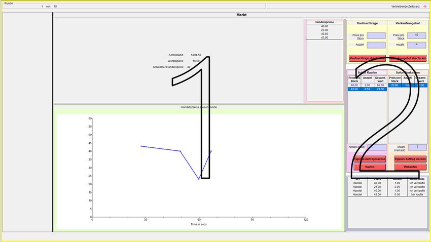
1       Introduction
Speculative bubbles are a major destabilizing factor for the economy and often have persis-
tent real consequences (e.g. Brunnermeier and Schnabel, 2016; Brunnermeier et al., 2020;
Gao et al., 2020). Perhaps one of the most well-known examples is the long-lasting eco-
nomic stagnation in Japan during 1991 to 2001 (“the lost decade”) after the burst of its
stock market bubble (Hoshi and Kashyap, 2004). There are many episodes of bubbles and
crashes in economic history such as the Dutch Tulip Mania, the Mississippi Bubble and the
South Sea Bubble (Garber, 2001), or the more recent Dot-com and U.S. housing bubbles
(Shiller, 2015). However, bubbles observed in cryptocurrency markets dwarf any major
historical bubbles in terms of magnitude and have been far more protracted (Bianchetti
et al., 2018; Cheah and Fry, 2015).
    Although cryptocurrencies were originally devised as a communication protocol that
facilitates decentralized electronic payments (Böhme et al., 2015), they are increasingly
recognized as an investment vehicle (Glaser et al., 2014). The first and perhaps most
prominent cryptocurrency is Bitcoin. Bitcoin alone constituted a market capitalization of
over $1 trillion at its peak price in 2021, which is comparable to the market capitalization
of all companies in the German DAX index. Choi and Jarrow (2020) carefully study
the prevalence of bubbles in cryptocurrency markets.1 Out of the eight most popular
cryptocurrencies, five clearly exhibit bubbles, including Bitcoin. It is puzzling why Bitcoin
exhibits such extreme bubbles since it does not generate any income such as dividends
or interest. Furthermore, it is different from commodities as it is intangible and has no
potential in being incorporated in the production of any further products in the way, for
example, gold does. Therefore, the conventional economic valuation measures cannot be
directly applied to cryptocurrencies (Burniske and White, 2017; Hong, 2017; Kristoufek,
2015). Nowadays, the majority of individuals who own cryptocurrencies are not holding
them as a substitute for cash (Baur et al., 2018), but rather for speculative purposes
(Yermack, 2015). As more investors hold cryptocurrencies in their portfolios, the risk of
speculative bubbles in cryptocurrency markets spreading to other financial markets and
ultimately to the real economy is increasingly likely (Guo et al., 2011; Manaa et al., 2019).
    What separates decentralized cryptocurrencies from conventional assets is the underly-
ing blockchain technology. Blockchain is a public ledger that records coin ownership, but
many permissionless cryptocurrencies such as Bitcoin require a consensus mechanism to
determine who has the right to add new information to the blockchain. Irresberger et al.
(2020) provide an extensive overview of the public blockchain ecosystem and find that al-
though there are hundreds of blockchains, only a few are of economic relevance. They show
that Bitcoin is by far the most adopted blockchain in terms of active users and that it is one
of the most relevant blockchains from an economic welfare perspective. Bitcoin’s blockchain
technology relies on the Proof-of-Work (PoW) consensus mechanism, commonly known as
mining, which is the most common consensus mechanism in cryptocurrencies (Gervais et al.,
2016). Bitcoin mining can be very costly as miners are required to solve a computationally
    1
     In order to determine bubbles, the authors apply the local martingale theory of bubbles, where the
fundamental value of a cryptocurrency can be interpreted as the currency’s liquidation value at the model’s
horizon (the buy and hold value).

                                                                                                         2
intensive problem but only those who succeed are allowed to add new information to the
blockchain. To encourage participation, the algorithm rewards miners with newly created
coins, which is also purposefully designed to be the only way to supply new coins to the
market. We offer a more detailed background on Bitcoin and its blockchain technology in
section 2.
We identify three defining features associated with the Bitcoin mining process that may
affect pricing. First, the reward of mining decreases over time such that in the long run, the
total supply of Bitcoin is limited by design. This is achieved by repeatedly halving a miner’s
reward at given intervals, which creates an increasing perception of scarcity. Second, the
rate at which new blocks are added to the blockchain is fixed (on average one block per
10 minutes). This implies that the supply is smoothed and cannot instantly respond to
demand shocks. Third, as Bitcoin gains popularity, competition for the reward of mining
increases (Alsabah and Capponi, 2020; Cong et al., 2021a). As more processing power
joins the mining network, the blockchain’s algorithm automatically increases the mining
difficulty, making mining more costly. Moreover, exceedingly high computational power
requirements for mining will disadvantage small individual miners, making it increasingly
infeasible for such individuals to mine bitcoins in a decentralized manner (Alsabah and
Capponi, 2020; Ferreira et al., 2019).2 This can further apply upward pressure on prices
as the channel through which individuals can acquire the asset becomes more exclusive as
compared to when mining is less centralized.
In this study, we analyze whether these key properties of Bitcoin mining can help ex-
plain its extreme price patterns.3 However, we are not precluding that other channels could
be causally related to pricing. Earlier studies have attributed Bitcoin bubbles on a suc-
cessful narrative (Shiller, 2019), or on darknet marketplace criminal activities (Foley et al.,
2019). More recently, Cong et al. (2021b) explain how the price volatility of cryptocurren-
cies may be causally related to endogenous user adoption. We instead focus on arguably
more fundamental reasons related to PoW based cryptocurrencies. In particular, we aim to
test whether the blockchain technology and supply scheme of Bitcoin, that we collectively
refer to as ‘mining’, contribute to explaining the commonly observed but otherwise not
adequately explained bubble phenomenon observed in cryptocurrency markets. Given the
abundant availability of naturally occurring financial data, there has been some effort in the
literature to understand the link between mining costs and prices of cryptocurrencies using
empirical studies. For instance, Bhambhwani et al. (2019) perform a multi factor analysis
2
The hash power small individual miners have is negligible compared to the global hash rate, thus,
making the expected reward proportionally smaller. This gives rise to mining pools for the purpose of
risk-sharing (Cong et al., 2021a). But even within such pools, the reward (net of fees) can be negligible for
an average individual miner as it is based on their individual hash power. Overall, the arms-race of mining
technology makes it infeasible for small individual actors to obtain Bitcoin through mining, who instead
have to rely on trading platforms.
3
While we focus on the case of Bitcoin, our analysis extends to cryptocurrencies relying on the PoW
mechanism such as hard forked variants of Bitcoin (Cash, Gold, Satoshi’s Vision), Ethereum Classic (ETC),
Dash, Litecoin, and Zcash. Our results do not apply to cryptocurrencies that adopt alternative consensus
mechanisms or without a supply limit such as Binance Coin, EOS, Ether, Monero (XMR), Ripple (XRP),
Stellar, and Tron (TRX). See Cong and Xiao (2020) for a comprehensive overview of the various categories
of cryptocurrencies.
3of 38 cryptocurrencies and conclude that the computing power (hashrate) and network
size (number of miners) influence cryptocurrency prices. Relatedly, Saleh (forthcoming)
theoretically studies the relationship between computing power and electricity consump-
tion, which is the main expense when mining. Hayes (2017, 2019) and Xiong et al. (2020)
empirically show that production costs, especially electricity cost, play an important role
in explaining cryptocurrency prices. However, such financial data and empirical studies
suffer from an absence of counterfactuals and it can be difficult to disentangle the effect of
mining from other (unobservable) factors that may also influence prices. Thus, we study
mining and mining centralization in a controlled laboratory environment, which allows us
to identify their causal effect on prices.
We are the first to design a controlled laboratory environment to study how the PoW
consensus mechanism affects pricing in cryptocurrency markets.4 The experimental method
has been successfully employed to test various financial innovations in the past such as the
pricing of financial derivatives (e.g., Oprea et al., 2009; Porter and Smith, 1995a; Noussair
et al., 2016) and algorithmic trading (Aldrich and López Vargas, 2020; Angerer et al.,
2019). Our experimental framework follows Smith et al. (2000) where market participants
can trade an asset with a random redemption value.5 In our setting, asset holders receive
no intermediate dividend payments but only a redemption value; the fundamental value
of the asset is constant and flat. It has been shown that such environments are not prone
to bubble and are, thus, suitable to use as a baseline (e.g., Cueva and Rustichini, 2015;
Kirchler et al., 2012; Noussair et al., 2001). There is no consensus how one should model the
fundamental value of a cryptocurrency, which is a much-debated issue in the literature and
has not yet been settled. For instance, Cheah and Fry (2015) and Shiller (2019) consider
Bitcoin worthless, as it is not a dividend-paying asset, while Biais et al. (2020) and Cong
et al. (2021b) suggest that Bitcoin (and other cryptocurrencies) has value because of the
transactional benefits it provides. These include acting as an alternative to fiat money when
the national currency and the banking system are in disarray or avoiding capital control.
Given the lack of consensus on evaluating the fundamental value of a cryptocurrency, we
follow the experimental finance literature and model our asset as a non-dividend paying
asset with a flat fundamental value that is not far from zero. This allows us to anticipate
the price dynamics of our baseline environment from the literature, thus, allowing us to
study the effect of mining in a controlled setting.
The experiment features a 2 × 2 design. The first dimension that we vary is the way
traders acquire the asset: either as a gift endowment or mining (Gift vs. Mining). In
the gift condition, traders receive assets as a gift and are also endowed with cash. In the
mining condition, traders do not receive any assets at the outset, but only cash. To acquire
assets, they need to spend some cash on ‘mining’ such that the asset can be generated for
4
To the best of our knowledge, there has not been any experimental study on cryptocurrency pricing in
a controlled laboratory environment. Perhaps the closest study to a controlled setting is Krafft et al. (2018),
who conduct an online field experiment and examine the effect of peer buying activity in cryptocurrency
markets on market liquidity. The authors deploy bot traders who initiate thousands of trades for less than
a penny for each of the 217 cryptocurrencies in their sample. Their results highlight the potential impact
of peer influence on liquidity in these markets.
5
A random redemption value is not crucial for bubble formation as shown by Porter and Smith (1995b)
who replace four point random payoffs by the expected value.
4them at a cost. The cost of mining increases as more units of the asset are mined in total.
The second dimension that we vary aims to capture the mining centralization, commonly
observed in permissionless cryptocurrencies where not all miners can mine cost effectively.
Specifically, along the mining condition, we vary if all or only half of the traders have access
to the mining facility (All vs. Half).
Our main results demonstrate that mining fuels bubbles. In the baseline treatment,
where mining is absent, there is no indication of bubbles. Price trajectories remain relatively
flat and close to fundamental value throughout the entire life of the asset, which is in line
with our conjecture based on the existing literature. Once mining is introduced, we observe
trading at prices of more than 200% above the fundamental value when all traders have
access to mining. More specifically, prices typically start below the fundamental value
but above the mining cost at the outset, then follow the mining cost for about 9 periods
(i.e. more than half of the trading periods) with some mark-up, before they peak and
subsequently crash. The mining costs seem to play a prominent role in determining prices
in periods where prices are hiking up. In the presence of mining centralization, our data
shows even more extreme patterns of bubbles and crashes. In particular, prices typically
trade already above fundamental value from the outset and soon after surge to a level
of almost 400% above fundamental value, resulting in a more protracted deflation of the
market. Prices decouple from both the fundamental value and mining cost at an early
stage. We observe that when half of the traders can only acquire the asset through the
market while there is a shared expectation that the mining cost will rise, traders are more
eager to purchase the asset early on, albeit at elevated prices. In both Mining treatments,
we find that mining activity goes beyond the social optimum suggesting that miners further
perpetuate mispricing in these markets.
Overall, the observation that mining and centralization of the mining technology fuel
overpricing in a controlled environment is a highly important result. Any effort put into
mining of cryptocurrencies is by design welfare harming (see Schilling and Uhlig (2019) for
a detailed argument). Furthermore, Auer (2019) explores what the future might hold for
cryptocurrencies and concludes that limitations of versions of the blockchain technology
which require costly mining will ultimately slow transactions down significantly. Similarly,
Easley et al. (2019) highlight the potential for inefficiencies and instabilities due to mining.
Relatedly, Huberman et al. (forthcoming) discuss various inefficiencies of the Bitcoin trans-
action process that stem from its mining protocol and propose alternatives that alleviate
these. On the other hand, it has been widely argued among popular media that mining will
become cheaper and faster with technological progress. However, as long as the price of
the cryptocurrency is attractive, miners will keep competing with each other and increase
their effort, leading to an unavoidable arms-race between miners (Alsabah and Capponi,
2020). The PoW algorithm adapts the mining difficulty according to mining effort ensuring
that the rate of block creation is stabilized at a predetermined level. Thus, even if only the
most cost efficient miners remain active, the mining cost would be sustained at high levels
due to the competition among miners. After all, competition is the only way to secure the
decentralized network. Overall, our results encourage the ongoing search for alternative
blockchain consensus mechanisms that are more efficient (e.g., Hinzen et al., 2020; Saleh,
forthcoming).
5The remainder of the paper is structured as follows. In section 2, we provide more
detail about the blockchain technology as employed by Bitcoin which is similar for many
cryptocurrencies. We then describe our experimental design in section 3. In section 4, we
present our hypotheses and report our results in section 5. Section 6 discusses the impli-
cations of our results and concludes. In the appendix, we report some additional analysis
and further experimental details, including the translated experimental instructions.
2 Background on Bitcoin & the blockchain technology
Against the backdrop of the 2008 financial crisis and deteriorated trust on the financial
system, the concept of Bitcoin was developed by Nakamoto (2008) as a decentralized peer-
to-peer (P2P) electronic cash system that is free from any entity’s control. The rules of
the money supply of Bitcoin are predetermined and fixed, which brings more monetary
discipline to the Bitcoin ecosystem. The information about the coin ownership of all par-
ticipants is recorded in a cryptographically secured public ledger, known as blockchain.
It contains all Bitcoin transactions since its inception. However, due to the absence of
a central administrator to manage the blockchain, a consensus mechanism is required to
determine who is allowed to add new information to the blockchain. The solution offered
by Nakamoto (2008) is called Proof-of-Work (PoW), which is widely used in other permis-
sionless cryptocurrencies. We focus here on the pertinent characteristics of PoW in the
context of Bitcoin for our purposes, for a comprehensive description of PoW and Bitcoin
mining see Gervais et al. (2016), Auer (2019) and Biais et al. (2019).
Under the PoW consensus mechanism, a new block can only be added to the blockchain
if its creator has successfully solved a computationally intensive cryptographic puzzle (i.e.,
finding a hash value that meets certain conditions). The process of solving this mathe-
matical problem is commonly referred to as ‘mining’. To compensate participants for their
contribution of computational power, the payment network rewards miners with certain
units of Bitcoin, which at the same time is the only way of introducing new coins to the
Bitcoin ecosystem. The level of the reward is set by the Bitcoin white paper and is halved
approximately every 4 years. Thus, the amount of new coins supplied to the market is
decreasing geometrically over time. As a result, the total number of Bitcoin supplied to
the market in the long run will reach a predetermined limit of 21 million coins.
Importantly, Nakamoto’s white paper also makes sure that these 21 million coins will be
supplied over a fixed number of years up until the year 2140. This is achieved by adjusting
the difficulty of the cryptographic puzzle for the PoW. In particular, “the [PoW] difficulty is
determined by a moving average, targeting an average number of blocks per hour [roughly
6 blocks per hour].” (Nakamoto, 2008, p.3). This ensures a smooth supply of Bitcoin in
the short-run. When mining activities intensify (diminish), the PoW difficulty increases
(decreases) accordingly. The increase in mining difficulty is also a protective measure for
the blockchain to ensure more security against attacks.
As Bitcoin and other PoW cryptocurrencies gain popularity, the number of computers
participating in its P2P network increases. With more computing power, the so-called
hash-power of the entire network increases. Accordingly, the mining difficulty increases
over time to keep its target block time, while miners compete against each other for the
6limited block reward. In recent years, the mining difficulty of a large set of cryptocurrencies
(which translates into monetary costs) has become prohibitively high for individual miners,
fostering the rise of professional miners. Professional miners have dedicated equipment
(Application-Specific Integrated Circuits, ASICs) to efficiently mine cryptocurrencies, while
individual investors can typically only purchase Bitcoin on the cryptocurrency exchanges
to include them in their portfolios.
These key properties of PoW discussed above are unique to Bitcoin and other similar
cryptocurrencies and are not shared by other conventional asset classes.6 Our experiment is
designed to test whether the defining features of mining cause the price volatility observed
empirically. Furthermore, our design also tests what further effect the centralization of
large professional miners can have on mispricing.
3 Experimental Design
3.1 Experimental Asset Market
Our basic experimental set up is close to Smith et al. (2000), which is similar to Smith
et al. (1988) but without intermediate dividends payment. Trading is done over 15 trading
periods. The asset that subjects trade only pays out a random redemption value of either
0, 15, 30, or 67 ECUs with equal chance at the end of the life of the asset, hence, the
fundamental value of the asset is flat at 28 ECUs. The flat but uncertain fundamental
value captures the plausibly divergent views on how cryptocurrencies are valued by different
investors. After the final trading period, the asset becomes worthless. Thus, the only
source of value of the asset is the redemption value, which is clearly communicated to the
participants. Trading is organized using an open book continuous double auction (Smith,
1962; Plott and Gray, 1990), which is the trading institution used in all our experimental
markets.7 Traders can freely post their own bids and asks or accept others’ proposals. We
do not allow for short selling or purchasing on margin. Trades can be made in whole units
or fractions (up to two decimals) of assets. Furthermore, there are no transaction costs for
trades nor interest payments for cash holdings.
We employ a 2×2 factorial design to examine the effects of mining and the centralization
of mining, summarized in table 1. We vary the nature of the asset influx to the market:
participants are either endowed with assets at the outset of the market (as a gift), or
they start only with experimental cash and can mine assets at a cost. The costly mining
incorporates the sticky and limited supply features of the PoW mechanism, employed by the
vast majority of cryptocurrencies. Mining implies that the cash-to-asset ratio (CAR) in our
mining treatments varies over time. We elaborate further on the specific implementation
of the mining process as well as on how we control the CAR across treatments below.
Additionally, we vary if all or only half of the traders are endowed with the asset in the
6
While the property of costly mining arguably shares similarities to natural resource extraction, cryp-
tocurrencies do not depreciate after usage and the speed of extraction does not depend on the miners
themselves (unlike, for instance, in the case of gold extraction, where it does depend on mining effort).
7
This type of trading organization is also commonly used in Bitcoin trading, see for example
www.bitcoin.de.
7Gift treatments, or are allowed to mine the asset in the Mining treatments. We conduct
9 market sessions for each of the four resulting treatments: Gift-All, Gift-Half, Mining-All
and Mining-Half.
Table 1: Summary of treatments
Centralization
All Half
Gift Gift-All Gift-Half
Asset Influx
Mining Mining-All Mining-Half
The Gift-All treatment is our baseline treatment in which all traders are endowed with
an equal amount of experimental cash and assets: 5700 ECUs and 20 units of the asset,
following Weitzel et al. (2019). This is a standard experimental asset market environment
similar to market A1 in Smith et al. (2000). Since each unit of the asset has a fundamental
value of 28 ECUs, the CAR, calculated as the total amount of money in the market over
the product of shares outstanding and fundamental value, is 10.2. This ensures that traders
will not be cash constrained if they are willing to pay elevated prices to acquire the asset
from the market.
The Mining-All treatment is identical to the baseline, except that traders are endowed
with only experimental cash, but no assets at the outset. If traders want to acquire assets,
they can either mine the asset at a cost, or buy the asset directly from the market, provided
that some units have already been mined. Mining operates concurrently with the asset
market. By contrasting Gift-All and Mining-All, we identify the effect of costly mining on
asset pricing. The cost of mining is an increasing function of the cumulated units of asset
mined (as cumulative expenditure). Traders can decide to spend up to 40 ECUs in each
period on mining. The mining cost per unit of asset is clearly known by everyone. Due
to the 40 ECU cap on mining expenditure, even when mining is profitable (for example if
assets are traded at prices higher than mining costs), there is a limit on how many assets
traders can mine per period. Thus, the smooth and limited supply features identified earlier
are proxied in the asset generation process. To compensate for mining costs and to control
the CAR across treatments (see details below), traders are endowed with slightly more
experimental cash as compared to the Gift-All treatment. Specifically, traders are endowed
with 5900 ECUs but no assets.
The cost of mining is characterized by the following function:
X χ
t̂
C xi,t = C (χt̂ ) = 5.4 · 1.5 40n (1)
i∈I, tFigure 1: Experimental implementation of asset supply vs. real-world supply schedule
Note: For both figures, the left vertical axis corresponds to aggregate asset supply, while the right vertical
axis corresponds to asset influx. The term asset subsidy in the right figure is commonly used to highlight
that new coins are introduced as a reward to successful miners.
all traders mine at full capacity, the cost function is calibrated to result in mining costs
at approximately the asset’s fundamental value at the fifth trading period. The exact
functional form is not communicated to participants, but they are clearly informed that
mining will become increasingly costly as more units are mined (see instructions in the
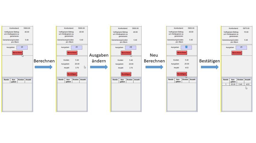
appendix). Mining costs adjust discretely at the start of each period. Participants can use
a calculator to estimate the mining cost for the next 4 periods by inputting their expectation
on mining expenditure per trader in the current period. The left panel of figure 1 presents
the asset supply evolution in our mining treatments over time. As a comparison, the right
panel of figure 1 presents the equivalent trend for Bitcoin. Notice how both figures exhibit
an exponentially decreasing supply over time.
Treatment Mining-Half is designed to capture the way cryptocurrency mining operates
in the real-world. For most cryptocurrencies, cost efficient mining requires a large number of
dedicated devices which are costly to acquire and utilize. This implies that many investors
have no option to cost effectively mine coins and, hence, are constrained to only obtaining
them through trading in the market. We study whether and how asset pricing is affected
when only half of the traders have the possibility to mine for assets, while the other half is
restricted to acquiring assets only from the market. With this treatment, we can identify
how centralization of the mining technology influences the asset pricing over and above
mining itself. However, the effect may also be attributed to asymmetry in holdings rather
than the mining protocol alone. In order to control for this, we also implement the Gift-
Half treatment where we randomly assign half of the traders to be endowed with both
assets and ECUs, while the other half do not receive any assets from the outset, but only
experimental cash.
In the Gift-Half and Mining-Half treatments, how traders are initially endowed depends
on their randomly assigned role. Half of the traders are assigned role A and the other
half role B. In Gift-Half, role A traders are endowed with 5140 ECUs and 40 assets at
the outset, while role B traders are endowed with 6260 ECUs but no assets. Note that,
given the expected redemption value of 28, the initial portfolios of traders in Gift-Half are
9equivalent to those of traders in Gift-All in terms of expected dividend value for both roles.
In Mining-Half, role A traders have a starting endowment of 5540 ECUs and zero assets
and are allowed access to the mining technology. Role A traders can potentially spend
up to 80 ECUs on mining in each period. We double their mining capacity per period to
allow for the market to have the same overall potential mining volume as the Mining-All
treatment. In the Mining-Half treatment, role B traders are endowed with 6260 ECUs but
no assets and have no access to the mining technology. Table 2 offers an overview of the
parameters for each treatment.
Table 2: Overview of parameters across treatments
All Half
Role A Role B
ECUs 5700 5140 6260
Gift
Assets 20 40 0
ECUs 5900 5540 6260
Assets 0 0 0
Mining
Mining Cap per Period
(in ECUs) 40 80 0
Miners are endowed with more ECUs than non-miners (5900 vs. 5700 & 5540 vs. 5140) to compensate
them for the mining cost, which is an increasing function of the cumulated units of asset mined so far.
These parameters are calbirated such that the CARs are comparable across treatments. See below for a
detailed description.
Special attention has been given to the calibration of the experimental parameters to
make our treatments comparable. While the CAR in Gift-All and Gift-Half is constant
throughout the trading periods, it varies over time in the Mining treatments (it is strictly
decreasing whenever mining takes place). We calibrate the parameters in a way that the
CAR of Gift and Mining treatments are similar – in figure 2 we depict the theoretical
expectation of the CAR development. Assuming every trader in Mining-All spends the
maximum amount possible (40 ECUs) in mining during each of the first five trading periods
and if no other transactions take place in the meantime, their holdings would be 5700 ECUs
and approximately 20 units of asset in period 5 (recall that the mining cost starts from
5.4 ECU in period 1, this will increase to 27.3 ECU in period 5 if everyone mines at full
capacity). This is essentially the initial endowment of traders in the Gift-All treatment.
Since the cost of mining is lower than the fundamental value of the asset during these first
five periods, the assumption of traders mining at full capacity seems reasonable. From
period 6 onwards, the mining cost would exceed the asset fundamental value, thus, risk-
neutral agents should refrain from further mining.8 Analogously, if all role A traders in
Mining-Half were to mine using their maximum allowance (80 ECUs) in each of the first
8
In this example, mining costs would increase from 27.3 to 41 ECUs per asset from the 5th to the 6th
period.
10five periods, they would reach (approximately) the initial endowment of role A traders in
Gift-Half.
Figure 2: Theoretical CAR across trading periods
30
20
CAR
10
0
0 5 10 15
Period
Gift-All, Gift-Half Mining-All, Mining-Half
Note: Assuming mining at full capacity in each period.
It is important to highlight some design choices we make. Firstly, we design the mining
process to be deterministic. Thus, we abstract away from uncertainty in the mining process
as miners can directly generate assets using ECUs. At any given point in time, the difficulty
of mining Bitcoin is public knowledge, while the direction, size and timing of any difficulty
updates in the future are not certain.9 Furthermore, miners can reduce the uncertainty
of successful mining through joining a mining pool (Cong et al., 2021a). These pools
share rewards of successful mining among all contributors, thus, reducing significantly any
uncertainty over reward of their costly effort. Similarly, in our design, subjects do not
face uncertainty about mining costs of the current period, but they can only estimate the
mining costs of future periods. This also helps to not overly burden our subjects with
increased complexity and uncertainty. Secondly, we choose to update costs as a function
of total expenditure. This allows for the natural interpretation of asset mining costs over
time: an increase by 50% in every period where mining is at full capacity. Updating costs
as a function of assets would require calculating how many assets are affordable to estimate
the mining cost.10 Finally, our mining cost implementation assumes identical costs for all
miners. In doing so, we abstract away from varying cost efficiency across miners around
the world. As we have already argued, irrespective of how cost efficient miners are, the
adaptive difficulty algorithm behind the PoW mechanism will always ensure that the rate
of new block creation and asset influx are both fixed at a predetermined speed. Thus, the
critical characteristic of PoW is this nature of a predetermined rate of asset influx which is
what we focus our design on. Additionally, modelling miners as having identical costs can
9
The difficulty level of mining is updated with every 2016 blocks added to the blockchain. The direction
of the difficulty update depends on the joint effort of all miners. The presence or absence of other miners
influences the difficulty level in the future. This is both through the exact timing of the next update, as
well as, through the new difficulty level after the update.
10
Figure A.1 in the appendix depicts costs as a function of total assets generated in our experiment.
11be seen as an approximation of a long-run environment where the less efficient miners are
crowded out.
All participants receive printed instructions to read at their own pace. We administer
a comprehension quiz which every participant has to pass after reading the instructions.
The quiz asks about features and parameters of the asset market.11 Before initiating the
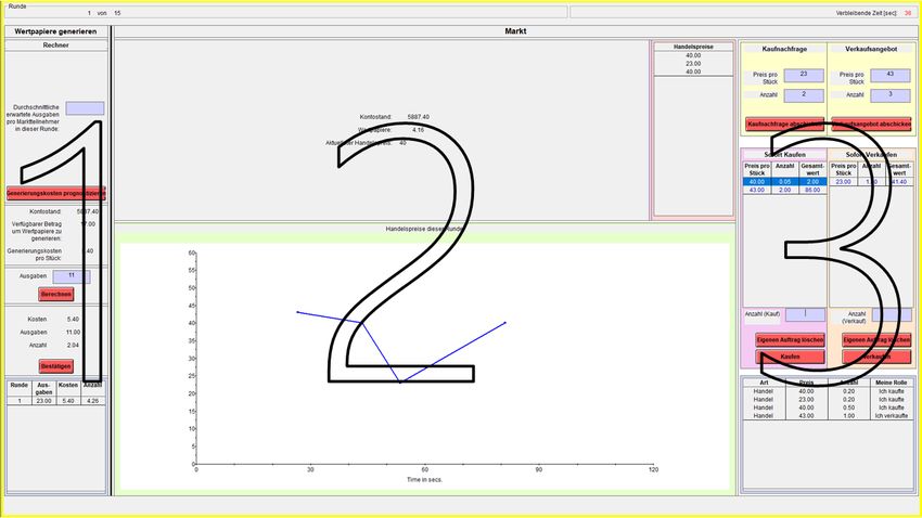
15 trading periods, participants go through three practice periods of 120 seconds each.
During these practice periods participants are encouraged to familiarise themselves with
the various functionalities of the platform. For example, they are encouraged to try out
asset generation and the corresponding calculator (if applicable) as well as placing ask/buy
orders and completing trades. The asset and ECU holdings are reset after these practice
periods (and practice periods do not count towards final earnings). The 15 trading periods
also have a duration of 120 seconds each. In Gift-Half and Mining-Half, the roles of traders
were randomly determined before the practice periods and were preserved for the trading
periods.
The basic asset market experiment design was pre-registered at the AsPredicted plat-
form of the Penn Wharton Credibility Lab. The pre-registration for the All treatments
with and without mining can be found at https://aspredicted.org/8hx2k.pdf and for
the Half treatments with and without mining can be found at https://aspredicted.org/
4w4hz.pdf.
3.2 Additional Controls
Before implementing our experimental asset market, in all sessions, we elicit a number of
individual traits and characteristics to be used as controls in the analysis.
Participants complete a short version of the Raven Advanced Progressive Matrices
(APM) test. The Raven test is a non-verbal test commonly used to measure fluid intelli-
gence, which is the capacity to solve problems in novel situations, independent of acquired
knowledge. In order to shorten the duration of this test, we follow Bors and Stokes (1998)
in using 12 from the total of 36 matrices from Set II of the APM. Matrices from Set II of the
APM are appropriate for adults and adolescents of higher average intelligence. Participants
are allowed a maximum of 10 minutes. Initially, they are shown an example of a matrix
with the correct answer provided below for 30 seconds. For each question, a 3 × 3 matrix
of images is displayed on the participants’ screen; the image in the bottom right corner
is missing. The participants are then asked to complete the pattern choosing one out of
8 possible choices presented on the screen. The 12 matrices are presented in the order of
progressive difficulty as they are sequenced in Set II of the APM. Participants are allowed
to switch back and forth through the 12 matrices during the 10 minutes and change their
answers. They are rewarded with 1 Euro per correct answer from a random choice of two
out of the total of 12 matrices.
We elicit Theory of Mind (ToM) using the Heider test (Heider and Simmel, 1944),
following Bruguier et al. (2010) and Bossaerts et al. (2019). ToM is the ability to infer
the intentions of other agents, which is especially important in market environments. The
Heider test involves a short film of moving geometric objects (two triangles of different size
11
We include the quiz questions in appendix E.
12and one circle). When watching the movie, one could personify the geometric objects as the
large triangle bullying the small triangle and the circle trying to intervene. To measure the
intensity of ToM, we pause the movie every 5 seconds and ask the participant to forecast
whether the two triangles are going to be further apart or closer together 5 seconds later.
People who are better able to imagine a bullying scene are more capable in forecasting the
future distance between the triangles (Bossaerts et al., 2019). The test results in a score of
0 up to 6 depending on how many of the 6 predictions participants are correct about. For
each correct prediction participants are rewarded with 50 cents.
Finally, we elicit risk preferences using an incentivized Eckel and Grossman (2008) task.
Once the asset market was completed, we administer a questionnaire for general demograph-
ics, comprehension of the expected value of the asset traded and previous experience with
cryptocurrencies.
3.3 Experiment Implementation Details
A total number of 286 participants took part in our experiment. We conducted 36 sessions
in total, with 9 sessions per treatment.12 Each market session had 8 participants, except for
two where we had 7 participants due to no-shows. The whole experiment was implemented
using z-Tree (Fischbacher, 2007) and the trading platform within z-Tree was implemented
using the technical toolbox GIMS developed by Palan (2015). To determine the redemption
value of our assets, we implemented a transparent randomization process which guaranteed
that each of the four buyback values would be assigned to exactly two participants.13 This
was done by having each trader physically draw from a deck of cards. The deck of cards
had 4 pairs of cards. Each pair corresponded to one of the 4 possible redemption values.
The cards were drawn privately without replacement by each of the 8 traders.
Our experimental sessions took place in the economics lab facilities in the University
of Heidelberg and Frankfurt University. Participants were mostly undergraduate students
from a variety of majors. Participants were recruited using ORSEE (Greiner, 2015) in
Frankfurt and SONA (www.sona-systems.com) in Heidelberg. The average payment was
approximately 18 Euros for 90 minutes. We include translated versions of the experiment
instructions in the appendix.
We summarize participant characteristics by treatment and role in table 3. Overall, our
treatments are balanced, in particular with respect to gender, which is important given the
recent finding that gender composition matters for market efficiency (Eckel and Füllbrunn,
2015).
4 Research Hypotheses
Our experimental design allows us to answer a number of research questions. Here, we list
four main hypotheses to be evaluated.
12
Table A.5 in the appendix summarizes dates and locations of implementation of each of our sessions
across all four treatments.
13
In the two sessions with only seven participants, one of the buyback values was assigned to only one
participant and which of the values would be assigned only once was part of the random procedure.
13Table 3: Characteristics of participants across treatments
Gift-All Gift-Half Mining-All Mining-Half
Role A Role B Role A Role B
Avg. Age 23.54 22.98 24.84 24.21 21.75 22.72
Proportion of Females 0.58 0.39 0.47 0.47 0.58 0.47
Avg. Crypto Experience† 1.72 1.94 1.81 1.73 1.67 1.92
Avg. Raven 8.22 7.78 7.83 8.11 7.61 7.78
Avg. Theory of Mind 3.36 3.5 3.56 3.61 3.58 3.56
Avg. Risk Choice 3.54 3.54 3.31 3.51 3.42 3.81
†
Crypto experience was elicited using a Likert scale from 1 (none) to 5 (very well).
Note: There are no statistically significant differences in these characteristics in pairwise comparisons across
treatments and roles (corrected for multiple testing using Bonferroni-Holm correction).
The setup of our baseline treatment, Gift-All, is closely related with market A1 of
Smith et al. (2000), where an asset with a flat fundamental is traded. Thus, we can
formulate hypotheses following from the established findings in the literature. In the Gift-
All treatment, we do not expect to observe bubbles and crashes given the results of Smith
et al. (2000). If traders are on average risk neutral, we should observe no trade, or trade only
at around the fundamental value (Palan, 2013). Moreover, our experimental design does not
entail frequent dividend payments as in Smith et al. (1988) with decreasing fundamentals,
or in Bostian et al. (2005) with a flat fundamental, where bubbles are commonly observed
(see also the discussion in Noussair and Tucker, 2016). Smith et al. (2000) report little
price deviation from the fundamental value and no sign of bubbles and crashes. However,
prices may be elevated and not track fundamental values perfectly, as the CAR is relatively
high at 10.2. Higher CARs have been shown to induce greater mispricing (Angerer and
Szymczak, 2019; Caginalp et al., 1998, 2001, 2002; Haruvy and Noussair, 2006; Noussair
and Tucker, 2016). In particular, Caginalp et al. (2001) estimate that each dollar per share
of additional cash results in a maximum price that is $1 per share higher.
Hypothesis 1. Prices in Gift-All do not exhibit a pattern of bubbles and crashes.
We next examine the treatment Gift-Half where only half of the traders are endowed
with both experimental cash and assets, while the other half are only endowed with exper-
imental cash. This endowment asymmetry may affect traders’ willingness to pay for the
asset. Weber and Camerer (1998) have suggested that traders tend to achieve a balanced
portfolio, implying that those starting with only cash may want to hold some assets as
well. More recently, Janssen et al. (2019) and Tucker and Xu (2020) find that bubbles are
larger and more common when traders start with an asymmetric endowment. However,
it should be noted that both studies adopt the Smith et al. (1988) framework, which has
been shown consistently in the literature that it is prone to bubbles (Palan, 2013). It is
ex-ante not clear whether the endowment asymmetry itself may trigger a price bubble in
an environment that rarely bubbles such as ours.
Hypothesis 2. Prices in Gift-Half are higher than prices in Gift-All.
14When mining is introduced, there are a number of behavioral reasons why prices may
decouple from the fundamental value, leading us to observe bubbles and crashes. First, the
cost function implies that mining will be more costly in the future as more units of assets
are mined, creating an expectation of a rising cost. Thus, the mining cost may serve as
a price anchor at different points in time. Additionally, it may also serve as a support of
prices in that traders may feel reluctant to sell the asset below the cost of acquisition due to
the sunk cost fallacy. Second, due to the expenditure cap on mining, the supply is sluggish.
This means that when demand is high in a given period, the supply of the asset cannot
accommodate the demand in a reasonably short period of time, thus, applying upward
pressure on the price (Saleh, 2019; Hinzen et al., 2020).
Hypothesis 3. Prices in Mining treatments are higher than prices in Gift treatments,
exhibiting a pattern of bubbles and crashes.
The Mining-Half treatment may further exacerbate this issue, as demand could be even
stronger when half of the traders can only purchase the asset on the market. Furthermore,
initially, there may just be a subset of miners who are selling assets that they mined. This
may make it easier for them to enjoy market power and maintain their asks at a relatively
higher price level given the limited competition. Lastly, relating to the recent findings of
Janssen et al. (2019) and Tucker and Xu (2020) we anticipate that the potential bubbles
will be larger in Mining-Half as compared to Mining-All,
Hypothesis 4. Prices in Mining-Half are higher than prices in Mining-All.
5 Results
5.1 Results on Market Level
Figure 3a depicts the trading prices of the asset across our four treatments. We report the
median price of each treatment based on volume-weighted prices from each market.14 We
first examine our Gift treatments. The price trajectories in figure 3a show that prices follow
the fundamental value relatively well across all trading periods regardless of endowment
centralization.
We formalize our analysis using a number of bubble measures, summarized in table
15
4. These indicators include RD, the relative deviation of prices from fundamental value
(normalized at 28) and RAD, the relative absolute deviation of prices from fundamental
value (normalized at 28), introduced by Stöckl et al. (2010). RAD measures how closely
prices track fundamental value, while RD indicates whether prices on average are above or
below fundamental value.
In table 4, the median value of RAD and RD in the Gift treatments is between 0.1
and 0.4, suggesting very modest mispricing. Thus, the Gift treatments provide us with a
14
Figure A.2 in the appendix is the equivalent figure depicting average prices instead of median prices,
offering similar conclusions. Additionally, figures A.3-A.6 depict the price trends separately for each of our
9 individual markets per treatment.
15
We report the exact formulas of all bubble measures in the appendix. In tables A.1-A.4 in the
appendix, we report these measures separately for each market of each treatment.
15Figure 3: Trading prices, volume and cash-to-asset ratio in all treatments
(a) Median of volume-weighted price per period
150
Volume-Weighted Price
100
50
FV
0
0 5 10 15
Period
Gift-All Gift-Half
Mining-All Mining-Half
(b) Session-median trading volume per period (c) Realized session-median CAR
80
30
60
Volume
20
CAR
40
10
20
0 0
0 5 10 15 0 5 10 15
Period Period
Gift-All Gift-Half Gift-All, Gift-Half Mining-All
Mining-All Mining-Half Mining-Half
16Table 4: Summary statistics of bubble measures by treatment
Gift-All Gift-Half Mining-All Mining-Half
median median median median
mean (std.dev.) mean (std.dev.) mean (std.dev.) mean (std.dev.)
RAD 0.4 0.1 1.0 2.1
0.5 (0.5) 0.5 (0.8) 1.9 (1.9) 2.3 (1.5)
RD 0.4 0.1 1.0 2.0
0.4 (0.5) 0.5 (0.9) 1.9 (1.9) 2.2 (1.5)
RDMAX 1.0 0.3 3.6 3.6
0.9 (0.6) 0.9 (1.4) 7.7 (10.7) 6.1 (5.2)
AMP 0.8 0.3 3.8 3.2
0.7 (0.3) 0.6 (0.6) 7.9 (10.7) 5.6 (5.0)
CRASH -0.5 -0.3 -2.9 -4.0
-0.6 (0.6) -0.7 (0.9) -7.5 (11.3) -6.2 (5.4)
TURN 0.2 0.2 0.2 0.2
0.2 (0.1) 0.2 (0.1) 0.2 (0.1) 0.2 (0.1)
LQ 0.6 1.0 0.5 0.8
0.8 (0.7) 5.5 (13.9) 0.7 (0.6) 5.2 (12.8)
SR 20.9 19.3 17.1 22.1
20.4 (4.4) 21.1 (4.9) 16.3 (3.5) 21.9 (3.5)
SPREAD 0.2 0.1 0.5 1.2
0.3 (0.2) 0.2 (0.3) 1.4 (2.3) 1.5 (1.2)
VOLA 0.2 0.1 0.3 0.4
0.3 (0.3) 0.2 (0.1) 0.3 (0.2) 0.5 (0.3)
Notes: RD: relative deviation of prices from fundamentals (normalized at the fundamental value of 28);
RAD: the relative absolute deviation of prices from fundamentals (normalized at the fundamental value of
28); RDMAX measures the overpricing of the peak period. AMPLITUDE captures the relative difference
of the pre-peak minimum price and the peak price in terms of magnitudes of the fundamental value and
CRASH compares the peak price to the minimum price post-peak (Razen et al., 2017). TURNOVER
measures the volume of trade. LIQUIDITY describes the volume quantities of open orders at the end of
each period, while SR is defined as the number of limit orders posted divided by the sum of limit and
market orders posted in a period. SPREAD measures the gap between buy and sell orders and VOLA
measures log-returns of all market prices within a period.
17Table 5: Exact Mann-Whitney-U tests comparing bubble measures across treatments
Gift-All Gift-All Gift-Half Mining-All
vs. vs. vs. vs.
Gift-Half Mining-All Mining-Half Mining-Half
RAD 0.546 0.004 0.003 0.666
RD 0.387 0.006 0.004 0.605
RDMAX 0.387 0.001 0.002 0.931
AMPLITUDE 1.079 0.002 0.036 1.000
CRASH 0.673 0.005 0.001 0.606
TURN 0.863 0.931 0.387 0.546
LQ 0.340 1.000 1.000 0.297
SR 1.000 0.050 0.666 0.006
SPREAD 0.340 0.006 0.000 0.136
VOLA 0.222 0.161 0.014 0.436
Note: We report the p-values for each test; we report in bold font whenever p-value ≤ 0.050.
good benchmark to study the effect of mining, with or without mining centralization. In
table 5, we report p-values of the Mann-Whitney U exact test to detect potential treatment
effects. We find no statistically significant differences in any of the bubble measures when
contrasting Gift-All and Gift-Half. This implies that endowment asymmetry by itself does
not ignite a bubble. Indeed, as observed in figure 3a, in neither of our Gift treatments
do we observe a pattern of bubbles and crashes. These observations lead to our first two
results:
Result 1. Prices in Gift-All treatment do not exhibit any pattern of bubbles and crashes,
offering supporting evidence for Hypothesis 1.
Result 2. We find no significant difference in overpricing between Gift-All and Gift-Half
treatments. Endowment asymmetry by itself does not ignite a bubble, thus, we reject Hy-
pothesis 2.
We next examine the Mining treatments. Figure 4 depicts trading prices only for the two
mining treatments together with their respective mining cost trends. In Mining-All, prices
initially start below fundamental value but above mining cost. The trajectory follows an
upward trend clearly parallel to the mining cost with a distinguishable mark-up. Overall,
prices continue rising for 12 periods before they crash in the last three periods. Similarly, in
treatment Mining-Half, prices go well above and beyond fundamental value. Prices seem to
decouple from the mining cost already within the first few periods and peak at even higher
levels. As seen in figures 3a and 4, the peak price of the median prices in the Mining-All
and Mining-Half treatments are more than 200% and close to 400% above fundamental
value, respectively. Our median representation is robust to potential outliers; in figure 5
we replicate figure 3a by systematically removing one of the 9 markets of each treatment
18Figure 4: Median volume-weighted price and mining cost per period in Mining treatments
150
Volume-Weighted Price
100
50
FV
0
0 5 10 15
Period
Mining-All Mining-Half
Realized Costs Mining-All Realized Costs Mining-Half
Figure 5: Range of prices per treatment per period
150
Volume-Weighted Price
FV 50 1000
0 5 10 15
Period
Gift-All Gift-Half
Mining-All Mining-Half
Note: Median volume-weighted price per period of all but one session in all treatments, which yields eight
graphs per treatment. We shade the area between the highest and lowest period prices per treatment, i.e.
all eight graphs of a treatment lie within the shaded area of the respective treatment.
19with replacement. The general price trajectories per treatment we report in figures 3a and
4 remain unchanged.
In table 5, when comparing the bubble measures of the Mining treatments to their
respective Gift treatment (Gift-All vs. Mining-All & Gift-Half vs. Mining-Half), we find
statistically significant differences (second and third columns). Specifically, mispricing is
significantly more pronounced in the Mining treatments as compared to the Gift treatments.
It is worth emphasizing that this result should not be solely attributed to the difference in
the CAR at the outset of the market. The cash endowment in the Mining treatments is
only around 4% higher than in the Gift treatments. Additionally, the CAR is already quite
high in the Gift treatments (10.2), thus, ensuring that traders are never cash constrained.16
Furthermore, the bubble observed in the Mining-All treatment peaks in the second half of
the trading periods, by which point the CAR is already lower compared to the CAR in the
Gift treatments.
Result 3. Overpricing in the Mining treatments is significantly greater than in the Gift
treatments, thus, we have supporting evidence for Hypothesis 3.
Table 6: Exact Mann-Whitney-U test in first and second half of trading
Mining-All Mining-Half p-values
RAD First half 0.60 2.20 0.011
Second half 1.33 0.81 0.436
RD First half 0.47 2.20 0.008
Second half 1.33 0.81 0.340
Finally, we are interested in identifying what effect centralization of the mining tech-
nology might have on asset pricing. To this end, we now focus on contrasting our two
Mining treatments. We find no significant difference when comparing the bubble measures
of Mining-All to Mining-Half when taking all periods into consideration (fourth column of
table 5). However, figure 4 suggests that there is a difference in the timing of the bubble
occurrence between the Mining-All and Mining-Half treatments. Table 6 compares our
Mining treatments, by splitting the trading periods in two halves. We refer to periods 1 − 7
as the first half and periods 9−15 as the second half. The bubble measures RAD and RD of
our mining treatments show a statistically significant difference in the first half of trading
periods.17 The market peaks earlier in treatment Mining-Half compared to Mining-All and
the bubble persists for a number of periods before prices crash to fundamental value. This
leads to our fourth result:
16
In fact, only 3 out of 144 traders in the Gift treatments are ever cash-constrained; two in Gift-Half
and one in Gift-All. These three traders used up approximately 95% of their ECU endowment in the first
three periods by purchasing at high prices and selling at low prices.
17
Since the bubble measures RDMAX, AMPLITUDE and CRASH are calculated with respect to the
peak period, they cannot be calculated when the trading periods are split in two.
20Result 4. The degree of overpricing of Mining-All and Mining-Half does not differ overall,
but prices in Mining-Half markets surge earlier than those in Mining-All markets. Thus,
we partly reject Hypothesis 4.
It is worth noting that the results that we report are not due to differences in trading
volumes across treatments. No treatment leads to a particularly thin market. Figure 3b
presents the average trading volume of each treatment across trading periods, albeit with
small differences in the initial periods. The Gift treatments appear to initially trade at
higher volumes but this difference quickly disappears. A plausible explanation for the initial
difference may be the fact that in the first few periods there are substantially fewer assets
available to trade in the Mining treatment markets. Figure 3c shows the median realized
CAR of our treatments across periods.18 Trading volume across the four treatments is
not significantly different once the CAR is similar (from 6th period onwards). This is
confirmed using a non-parametric test of comparing average trading volumes of periods 6-
15 across the four treatments (Mann-Whitney-U test of Mining vs. Gift, p − value = 0.393;
Mann-Whitney-U test of All vs. Half, p − value = 0.800).
5.2 Over-expenditure on Mining
Given the discussion in the literature on how effort spent on mining can have harmful
implications on overall welfare (e.g. Auer, 2019; Schilling and Uhlig, 2019), we want to
understand if mining expenditure is executed optimally in the Mining treatments. From
figure 4, given the rising mining costs, it can be inferred that mining expenditure is not
halted once costs exceed the fundamental value of the asset. At the individual level, such
behavior can be rationalized since market price exceeds mining cost. However, from a
social planner’s perspective, mining at a cost above fundamental value is detrimental to
overall welfare. We find spending on mining is more than the social optimum, with market
over-expenditure on mining across different sessions ranging from 25% to about 133% in
the Mining treatments (median session over-expenditure in Mining-All and Mining-Half is
53.5% and 55.0%, respectively). However, there is no statistically significant difference in
over-expenditure on mining between the Mining-All and Mining-Half treatments (Mann-
Whitney-U test, p − value = 0.474).
5.3 Additional insights from the order book
To gain some insight into what leads to the bubbles we observe, we now focus on analyzing
the order book. We want to identify whether trades are mostly driven by the demand-
side or the supply-side of the market and in particular, whether the bubbles appear to be
supply- or demand-driven. To this end, we analyze whether the transactions are mostly
initiated by buyers or sellers and we separately plot bids and asks proposed by traders.
Figure 6 summarizes the results. First, figure 6a shows that approximately three quarters
of accepted trades are consistently originating from asks in all four treatments. That is,
18
The figure reports the median realized CAR over the 9 markets implemented for each of the four
treatments.
21You can also read