Marrying up: field experimental and household survey evidence of competitive search for a taller and richer spouse

Marrying up: field experimental and household survey evidence of
 competitive search for a taller and richer spouse

 May 31, 2021
 Pierre-André Chiappori, David Ong, Yu (Alan) Yang and Junsen Zhang*

 Couple’s heights tend to match. However, whether such matching is for the sake of
 height or the many desirable traits associated with stature (e.g., income) is unclear.
 We contribute novel experimental and empirical data to identify gender differences
 in search behavior for mate height and income. We recorded clicks on profiles with
 randomly assigned height and income information on a major online dating website.
 These clicks reveal that taller men prefer taller women. By contrast, women not only
 prefer taller men but also higher income men, permitting the calculation of their
 willingness to pay (WTP) for mate-height. Surprisingly, short women have the
 highest WTP for mate-height. We confirm this heterogeneity in preference for mate-
 height by applying the method of Chiappori et al. (2021) for multidimensional
 matching to data on married couples. Short early mothers drive these results. Our
 evidence is consistent with short women attempting to match non-assortatively to
 increase the height of their children. We contribute to the search and matching
 literatures with one of the few papers on multidimensional search which integrates
 directed online search behavior with outcome data on marriages.

 Key Words: directed search, matching, marriage, anthropometry, height, online dating, field
experiment, gender differences
 JEL Codes: C93, J01, J12

 *
 Pierre-André Chiappori (corresponding author), pc2167@columbia.edu, Columbia University; David Ong, dvdong@gmail.com, Jinan
University-Guangzhou; Yu (Alan) Yang, alan.yang@wisc.edu, University of Wisconsin-Madison; Junsen Zhang, jszhang@cuhk.edu.hk,
Department of Economics, Chinese University of Hong Kong

1 / 58

 Introduction

 Couple’s heights tend to match (Weitzman & Conley, 2014). However, whether such
matching is for the sake of height or the many desirable traits associated with height as indicated
by the positive association with the synonym for height, “stature” is yet to be established. Stature
is correlated with many desirable traits (RH Steckel, 1995), especially for males: cognitive ability
(Case & Paxson, 2008), non-cognitive ability, e.g., self-confidence (Persico, Postlewaite, &
Silverman, 2004), health (Lundborg, Nystedt, & Rooth, 2009), educational attainment, occupation
and industry (Case, Paxson, & Islam, 2009), career prospects (Herpin, 2005), happiness (Deaton
& Arora, 2009), and through these factors, or by itself, socioeconomic status (Cavelaars et al.,
2009; Hatton & Bray, 2010; Peck & Lundberg, 1995; Singh & Mitra, 2017; Walker, Shaper, &
Wannamethee, 1988) and income (Case & Paxson, 2008; Gao & Smyth, 2010; Harper, 2000;
Heineck, 2005; Persico et al., 2004). Moreover, stature, unlike those other traits, is readily
observable and may, therefore, function as an important basis for the initial sorting among couples.
Indeed, there is evidence that taller men are more attractive to women (Hitsch, Hortaçsu, & Ariely,
2010b; Oreffice & Quintana-Domeque, 2010; Pierce, 1996; Tao & Yin, 2015).
 Given the associations between height and other desirable qualities, assortative matching on
height alone could contribute to the increase in economic inequality across families (Schwartz,
2013; Schwartz & Mare, 2005) and across generations for associated traits, because height, as well
as being readily observable to potential mates, is also highly heritable (McEvoy & Visscher, 2009;
Stulp & Barrett, 2016). The heritability of height ranges from 0.80 in developed countries to 0.60
in developing countries, like China, which has a heritability quotient of 0.65 (Li et al., 2004). In
developing countries, nutrition and other environmental factors could exert a greater influence on
realized height based on genetic potential. Assortative mating on height alone could, therefore,
also contribute significantly to the intergenerational persistence of inequality and the continued
association between height and social class, even more so than birth weight (Currie & Moretti,
2007). However, despite the importance of assortative mating by height, there is little work in the
economics literature on how people might search and match on height, and whether such matching
is the result of a preference for mate-height or the other associated factors (SE Black & Devereux,
2011).
 We contribute to the understanding of the preference for mate-height by randomly assigning
heights and incomes to 360 unique artificial profiles on a large online dating website in China. The

2 / 58

heights were one standard deviation below, at, or above the average heights of each gender: 160
cm for women and 172 cm for men in the cities of the experiment.1 These we refer to respectively
as “short”, “medium” and “tall” heights. We also randomly assigned these profiles “low”,
“middle”, and “high” incomes. We then counted “visits” or clicks on abbreviated profiles from
search engine results, which display the height and income information. Because we independently
manipulated income and height with online dating data, we can identify the effect of height on
visits separated from income and income separated from height, and thus, cleanly test for the pre-
matching (in other words, before the opposite sex’s preferences and intra-sexual competition
becomes significant) willingness of men and women to tradeoff between mate-income and height.
 First, we show that both men and women prefer tall members of the opposite sex
independently of income, educational attainment, and even beauty, and health--as revealed through
profile pictures. Second, we confirm prior work that men are indifferent to women’s incomes,
whereas women prefer higher income men in China (Ong & Wang, 2015). Thus, we can find
women’s tradeoff between mate-income and height. Moreover, our design allows us to test for the
possibility that women (men) of different heights may vary in their willingness to pay for mate-
height. To test for potential heterogeneity among women (men) in their preferences for mate-
height, we calculated how much women (men) of different heights are willing to pay for mate-
height at each of the male (female) profiles’ heights.
 Surprisingly, women's preference for mate-height, as reflected in how much mate-income they
are willing to give up for it, in other words, the willingness to pay for mate-height–what we term
as ‘willingness to pay’ (WTP) for mate-height—forms a “U-shaped” envelope on their height. For
short men, an incremental increase in their height significantly increases their attractiveness to
short women in terms of the income the women are willing to give up for an incremental increase
in the men’s height. An incremental increase in short men’s height increases their attractiveness
less to medium women than it does to short and negligibly to tall women. However, we observe
the reverse ranking of WTPs among women for men’s height at the tall men’s height. An
incremental increase in the tall men’s height significantly increases their attractiveness to tall
women, but less so to medium, and a negligibly to short women. Moreover, short women’s WTP
at the short men’s height is greater than tall women’s at the tall men’s height. Hence, whereas

 1
 These are: Beijing, Shanghai, Chengdu, and Shenzhen. Adult men are on average 5 cm shorter in China than in the US, where they are on
average 177 cm in height. Adult women are 3 cm shorter in China than in the US, where they are on average 163 cm in height.

3 / 58

men’s preference is assortative on mate-height in the sense that the taller the man, the stronger his
preference for height, women’s preference for mate-height is non-assortative; the shorter the
woman, the stronger is her preference for height.
 We test the predictiveness of these preferences revealed in online dating data by analyzing the
income and height characteristics among married couples using the Chinese Family Panel Studies
(CFPS) household survey data. To find the WTPs of height across women of different heights for
these realized matches that resulted in marriage, we used the methodologies developed by
Chiappori, McCann, and Pass (2021) for multidimensional matching and that of Vella (1993) to
control for unobserved selection in our simultaneous equations model. Consistent with the U-
shaped envelope of WTPs found with online dating data, the WTP of height for short wives is
significantly higher than medium and insignificantly higher than tall wives. For short wives, a 1
cm increase in husband height is equivalent to between a 14-17 percent increase his income, which
is more than twice that of the husband of the medium wife.
 We hypothesized that this demand for a taller husband, which at some level is inversely related
to their height if the women are short enough, can be driven by short women’s desire for taller
children. Such a desire may reflect their wish for their children to escape their own hardships from
widespread height discrimination in China (Kuhn & Shen, 2013). One way to test for this is to
look at the WTP for height among women who have children earlier when men are more plentiful.
 Confirming this conjecture, we find that whereas all early mothers’ WTP for mate-height
increases with the availability of men, as measured by the local sex ratio, short early mothers
increase weakly more than medium and significantly more than tall early mothers. Short early
mothers are willing to give up 3.8 percentage points more income for every 1 cm increase in height
than medium mothers. We find none of these effects for fathers.
 Our findings with online dating and marriage data reject a general preference basis for
assortative mating by height. Instead, they suggest that women’s preference for mate-height is
reference dependent. However, unlike the case with a reference-dependent preference (RDP) for
mate-income, where high-income women exhibit the strongest preference for high-income men
(Ong & Wang, 2015; Ong, Yang, & Zhang, 2020), women’s preference for male height may be
inversely related to their height if they are short. Our findings are also consistent with the
hypothesis that women’s marginal utility for mate-height may reflect concern for the height of
their children, and moreover, that there may be a gender difference in intergenerational altruism.

4 / 58

 Given that short women have the highest intensity preference for mate-height, prior work on
reference-dependent preference (Ong et al., 2020) suggests that they could lose out in the
competition for taller men when those men become more plentiful, because the increase in the
numbers of those men may disproportionately increase the competitive entry of other women who
might have been satisfied with shorter richer men when taller poorer men were less available.
Indeed, only short women’s probability of marriage decreases with local sex ratios, both relative
to medium women and in absolute terms. A 10 percent increase in the sex ratio decreases the
marriage probability of short women by 1.8 percentage points in absolute terms and 5.7 percentage
points compared with medium women, who are more likely to marry when sex ratio increases.
 The local sex ratio does not affect older mothers, including wives who are not mothers, up to
the age of 45, in their willingness to pay for husband height. These findings extend previous work
on RDP (Ong et al., 2020), which focused only on income by showing that women also have an
RDP for mate-height and one that may be inversely related to their height.
 We contribute to the search and matching literatures with one of the few papers on
multidimensional search which integrates directed online search behavior with outcome data on
marriages. We identify a vertical preference for mere height on the part of both men and women.
In the case of women, we can calculate their WTP for mate height. Moreover, we show a gender
difference. While men’s preference for mate height increases on their own height. Women’s
preference for mate height, as indicated by their WTP, forms U-Shaped envelope on the men’s
heights. We confirm prior work within directed search framework showing that those who value
matching with mate characteristic the most may lose out to competitive entry with the greater
availability of those mates (Ong et al., 2020).
 An important concern to rule out for identifying preferences is to rule out possible strategic
behavior. In our case, because visits to profiles are visible to owners, the visitors may condition
their visits on expectations of likely reciprocal visits of the owner of the profile (Bapna,
Ramaprasad, Shmueli, & Umyarov, 2016; Cheremukhin, Restrepo-Echavarria, & Tutino, 2020;
Egebark, Ekström, Plug, & van Praag, 2021).However, we can rule out this confounder because
we find, like Ong and Wang (2015), find that men of all income levels click on women of all
income levels with equal probability. This pattern is not consistent with a strategic motive to avoid
rejection implied by non-reciprocation of visits. Such a motive would imply higher rates of visits
to higher income women from higher income men, which we do not find. We identify women’s

5 / 58

preference for taller and higher income men. Strategic avoidance of rejection would predict that
short women click rate on taller men should be lower than tall women. However, we find that short
women’s WTP for height is greater than tall women’s at the short and medium man’s profile
height. So, while we cannot rule out strategic avoidance of non-reciprocity on the part of short
women at the tall man, we can at the short at the medium men’s heights.

 A fear of rejection could, however, bias the size of coefficient downward resulting in an
 underestimation of the intensity of short men’s and women’s preference for taller mates.
 While we do not observe the degree of strategic behavior across height and income upon
 which our calculation of the WTP depends, our main finding is that WTP is U-shaped on the
 women’s height. Short women have the highest WTP, followed by the medium women at the
 short and medium man. Only at the tall man is the pattern of WTP consistent with strategic
 behavior.2Related literature

 A vast literature on matching has grown out of Becker’s (1973) seminal work on the reasons
why people form families (Schwartz, 2013; Schwartz & Mare, 2005). Recently, Becker’s theory
has given rise to a nascent literature on matching by anthropometric characteristics such as body
mass (Oreffice & Quintana-Domeque, 2010) and height. Prior empirical studies suggest that
women prefer taller men in online dating and marriage data in the US (Hitsch, Hortaçsu, Ariely,
Hitsch, & Ariely, 2010), in speed dating data (Stulp, Buunk, Kurzban, & Verhulst, 2013; Stulp,
Buunk, & Pollet, 2013), and in marriage data from the UK (Belot & Fidrmuc, 2010). Apart from
the aforementioned correlation between height and other desirable qualities, especially in men,
mere height in men is considered an attractive feature, and attractiveness increases earnings in
Western countries (Hamermesh & Biddle, 1994). Height has less of (Case & Paxson, 2008) or
insignificant (Heineck, 2005) effect on women’s wages. Height raises earnings for both genders

 2
 Prior attempts to identify the preference for actual or potential mate incomes are consistent for women, but conflicting for men. Generally,
women prefer higher absolute and relatively higher income men (Hitsch, Hortaçsu, & Ariely, 2010a; Ong & Wang, 2015). There is some evidence
that men may also prefer higher income women, though the preference is weaker than women’s for higher income men (Hitsch, Hortaçsu, & Ariely,
2010a). Indeed, men may be indifferent to women’s actual (Ong & Wang, 2015) or potential income, as indicated by educational attainment (Neyt,
Vandenbulcke, & Baert, 2019; Ong, 2016). There is even evidence that men are averse to higher potential income women (Egebark et al., 2021;
Fisman et al., 2006).
 Men’s ambivalence towards higher income women might due to the demonstrated lower relationship stability if their wife out earns them
(Bertrand et al., 2015; Folke & Rickne, 2020; Foster & Stratton, 2021; Goussé, Jacquemet, & Robin, 2018). This lack of stability may be due to
women seeking mates who can compensate them for the labor market opportunity cost of marriage (Ong et al., 2020). In that case, men should
tradeoff the consumption gains afforded with a higher income mate with the greater risk of dissolution of the relationship. Recent evidence using
regression discontinuity analysis at exogenous admissions cutoffs suggests that the high level of correlation between couple’s educational
attainment is largely due to meeting opportunities, in particular, sorting by educational institutions rather than preferences (Belot & Francesconi,
2013; Kirkebøen, Leuven, & Mogstad, 2021; Nielsen & Svarer, 2009). Hence, the correlation we find in married couple’s education and income
could be driven by women’s preferences alone or by sorting by educational institutions.

6 / 58

because it is an indicator of increased human capital in China (Gao & Smyth, 2010) and Taiwan
(Tao, 2014). This correlation between height and human capital may contribute to the widespread
labor market discrimination by height in China (Kuhn & Shen, 2013). All of the advantages
associated with height may persist for many generations, due to the heritability of income,
educational attainment (Schwartz & Mare, 2005), and height (Cole, 2003), so that height becomes
the visible indicator of class (Cardoso & Caninas, 2010; Harper, 2000; Hatton & Bray, 2010;
Singh-Manoux et al., 2010), and therefore, a possible basis of assortative matching by class, and
thereby, a contributing factor to the continued stratification of societies by socioeconomic status.
Despite the adoption of communism in China, class exerts a considerable influence on life
outcomes (Gregory Clark, 2014), in addition to educational attainment and occupation (Jia & Li,
2016).
 Unsurprisingly, height increases mating success and fertility for men in Taiwan (Tao & Yin,
2015). However, the effect of height alone in matches can be difficult to identify, owing to the
previously mentioned correlations between height and many other desirable traits. Women (men)
may be reacting to these other characteristics of men (women), e.g., income when they appear to
be matching on height. More important for the social science of marriage matching is the inverse
possibility that a preference for mate-height can be exerting a significant but unobserved influence
in speed dating or marriage data. Height can be the driving factor in women’s apparent preference
for more ambitious men (Fisman, Iyengar, Kamenica, & Simonson, 2006), who may well be taller
than the average man. Conversely, height can be the basis for less ambitious men’s dis-preference
for more ambitious women, who may be taller than the average woman, and even the average man.
 The “chemistry” of spontaneous characteristics that arises when couples meet presents a
further problem for disentangling the preference for mate-height from other preferences in
empirical data. For example, a woman’s reaction to men who happen to be taller than her may
make her more attractive to them. Her pupils may dilate (Tombs & Silverman, 2004). Her voice
may soften (Fraccaro et al., 2011). Hormonal changes may also occur on meeting (Grillot,
Simmons, Lukaszewski, & Roney, 2014; López, Hay, & Conklin, 2009), which may increase the
attractiveness of couples to each other at that moment in ways that are not captured by standard
measures (Fraccaro et al., 2011). See Van Anders, Grey and Anders (2007) for an academic and
Alexander (2012) for a popular survey of the academic literature. Women’s preference for taller

7 / 58

men, which could make them more attractive to those men, could then induce a preference in taller
men for shorter women.3
 The self-reported preferences revealed in surveys may seem a natural remedy for these
problems of separating height from non-height preferences. However, surveys of preferences for
ideal mate characteristics have not been predictive of revealed preferences based on speed dating
experiments (Eastwick, Luchies, Finkel, & Hunt, 2014). Indeed, there is no reason to expect that
people can separate their preferences through introspection any better than social scientists can
from their choices. For example, subjects may always imagine tall men as also being more
healthy/handsome/athletic/intelligent, because that is true of the tall men they know. As a
consequence, they misreport a preference for mate-height when they actually cared about those
other characteristics. Beyond confusion in the understanding of one’s own preferences, people
may not be aware or may be reluctant to reveal their preferences in surveys. In an empirical study
of online dating behavior, Hitsch et al. (2010) find a within-race preference revealed by women in
their first contact emails to men, which was not revealed by the women’s stated preferences.
 These simultaneity and omitted variable problems in identifying non-height mate preferences
from speed dating experiments are exacerbated in marriage data. Spontaneous characteristics from
the chemistry that arises from well-matched statures (or the lack thereof from mismatched statures)
could give rise to permanent relationship advantages (or handicaps). Height alone, or through its
correlation with income, can contribute to the diminished marital satisfaction in couples in which
the husband has a lower income than his wife, but in which relative heights were not controlled
for (Bertrand, Kamenica, & Pan, 2015; Brown & Roberts, 2014). Few studies have attempted to
separate the effect of income and height on matching behavior. Belot and Fidrmuc’s (Belot &
Fidrmuc, 2010) empirical study of the effect of height in cross-ethnic marriages using real marriage
data controlled only for educational attainment. To our knowledge, only Hitsch et al. (2010)
controlled for mate-income when they tested for the effect of height on attraction.
 We overcome these endogeneity and omitted variable issues by identifying gender differences
in preferences for mate-height ex-ante to any interactions in a field experiment on one of China’s
largest online dating websites. Our field experiment is in the tradition of the large correspondence
studies literature on labor market discrimination. To our knowledge, this is the first field

 3
 Note that this problem is distinct from the well-recognized problem of men seeming to prefer women who are shorter than themselves because
they expect higher rates of rejection from women who are taller than themselves.

8 / 58

experimental study of the effect of height and income on mate preferences with random
assignments of both.
 The mutual selection of married couples presents a significant challenge for identifying the
willingness to pay WTPs for mate characteristics of each member. Chiappori, Oreffice, and
Quintana-Domeque (2012) derive an index condition theoretically which allowed them to identify
the couple’s WTP for their mate’s BMI empirically. Chiappori, McCann, and Pass (2021) extend
the theoretical results in Chiappori et al. (2012) by developing a theoretical basis for the
identification of the WTP of couples even if the index condition is not met. Based on the theoretical
results of Chiappori et al.’s (2021), we extend the empirical results in Chiappori et al. (2012) by
testing for whether men’s and women’s willingness to pay for mate-height in China varies with
their own height. We do this by estimating the WTPs for men and women for three height groups
and applying the estimator of Vella (1993) to control for unobserved selection by the spouse across
different height groups on our simultaneous equations.

 Online Dating Field Experiment

 Experimental Design

 We conducted our experiment on one of the largest online dating websites in China, with a
reported membership of 100 million in 2016. This website advertises itself as a matchmaking
website for white-collar professionals between the ages of 25 and 45 years of age. Prior work (Ong
et al., 2020) on website users in a similar set of cities suggests that the users of this website are
demographically similar to the surrounding population of singles in the same city. Users can create
a profile without a paid membership. These profiles must include demographic (e.g., age and
gender), socioeconomic (e.g., income), and physical characteristics (e.g., height) information, at
least one photo, and a free-text personal statement. Such requirements are common to most online
dating websites. Users may also add information, particularly, verifiable information, which would
increase the “credibility” of their profile. 4 Users can browse, search, and interact with other

 4
 The credibility of the profile is indicated by a score. This score can be increased with phone verification of the registered phone number,
a government-issued ID, extra photos, email and phone verifications…etc. All our profiles have a low credibility score, because they have only
phone verification and one photo. However, the low score does not appear in user search results, and hence, would not affect visits to our profiles.
To affect visits, users would have to search specifically for low-credibility profiles. Even then, such searches would not affect visit rates across our
profiles, which is the basis for our findings.

9 / 58

members after registration. Typically, users begin by inputting their preferred age range and
geographic location of partners into the search engine. The query returns a set of abbreviated
profiles which include: ID, picture, nicknames, age, city, marital status, height, income, and the
first two lines of a free-text statement. Users can then click a link and “visit” the full profile.5 They
can signal interest for free. However, emails require a payment of 10 CNY/month membership at
the time of the experiment, when 1 USD was approximately 6 CNY. We only recorded visits.
 We constructed 360 (180 for each gender) profiles by collecting nicknames, pictures, and
statements from inactive real profiles from another website that would have automatically hidden
them after a month of inactivity.6 We posted our constructed profiles for 24 hours to a randomly
assigned city, which is unlikely to be the same as that from which the depicted user originated. At
the end of the 24 hours, we closed the account.
 For the profile’s fixed traits, we assigned male profiles the age of 27 and female profiles the
age of 25, which are the average ages of marriage of men and women, respectively, in China.
Birthdays were within eight days of each other and under the same zodiac sign. We assigned our
profiles a college educational attainment, a marital status of “single with no children”, and no
house ownership.7
 The main treatment consisted of a block-random assignment design with three heights and
three incomes for each gender. “Short” male profiles are 166 cm in height, one standard deviation
below the average of “medium” male profiles, which are 172 cm (Zhang & Wang, 2011). “Tall”
male profiles are 178 cm, one standard deviation above medium. These male profiles were block-

 5
 Visits are necessary for any further interactions. They are costly in so far as they require time. Hence, we expect people to reveal their
preferences through their observed tradeoffs between profiles to visit. On the other hand, we do not expect these visits to be made strategically to
avoid rejections. A visit reveals only an ex-ante desire to see the full profile, and not necessarily an ex-post desire for more interactions. Thus, we
also do not expect visits to be made strategically to avoid humiliating rejections, because visits do not imply an offer to be rejected.
 6
 To our knowledge, no legal restrictions exist on the noncommercial use of user-created content uploaded to social media websites in China.
We assume that such restrictions, if they exist, are weaker in China than in the United States, where our research activities would also fall under
the “fair use” exemption to the US copyright law. Major US social media websites explicitly announce terms of use that effectively makes uploaded
user-created content public domain. See, for example, “publish content or information using the Public setting” in
https://www.facebook.com/legal/terms.
 We do not expect users to provide more than a brief glance at our profiles, which contain little information beyond what was already revealed
in the search engine results. Indeed, no one pursued further contact with any of our profiles. Moreover, our profiles are spread out among many
other profiles on any given day. They are also spread out across many days. Users of this website are unlikely to encounter o ur profiles more than
once (if at all).
 Chinese universities, similar to European universities, do not have IRBs to approve the ethics of experiments. However, to the best of our
understanding, our design falls under the “minimal risk” exemption from IRB approval. “Minimal risk means that the probability and magnitude
of harm or discomfort anticipated in the research are not greater in and of themselves than those ordinarily encountered in daily life o r during the
performance of routine physical or psychological examinations or tests.”
 See here: http://www.virginia.edu/vpr/irb/sbs/resources_regulations_subparta.46.101.html#46.102(i)
 7
 30-40 years old men who are college graduates in Beijing and Shanghai earn approximately 8k/month. The lowest income profile in our
experiment is 3-5k/month, which is approximately between the 20th and the 50th percentiles, according to CFPS data for 2010. However, the
sample is quite small (44 observations for male 30-40 years old college graduates in Beijing and Shanghai). The comparable Census data for mate-
income distribution in 2010 is unavailable.

10 / 58

randomly assigned one of three levels of incomes: 3-5, 8-10, 10-20 (1,000 CNY).8 These incomes
are slightly higher than the median for this website to make our profiles more attractive to potential
female visitors.
 “Short” female profiles are 155 cm in height, one standard deviation below “medium”, which
are 160 cm (Zhang & Wang, 2011), which are in turn one standard deviation below tall, which are
165 cm in height. These female profiles were block-randomly assigned incomes: 2-3, 3-5, 8-10
(1,000 CNY). 3-5 is the mean income level for women of this age group on this website. In
summary, we had 20 profiles for each combination of income and height in our 3×3 design for a
total of 180 profiles for each gender. Thus, with these treatments, we constructed 360 profile “slots.”
We then randomly assigned according to gender 360 pictures, nicknames, and personal statements
to these 360 slots.
 Users can rank the profiles of other users by the registration time, login time, age, number of
photos, the credibility of the profile, and income in the website’s search engine. The website also
highlights randomly selected (so far as we can tell) new profiles. Neither should affect our results,
because all of our profiles had statistically identical characteristics.
 Users could view our profiles’ picture, nicknames, age, city, marital status, height, income,
and the first few lines of a free-text statement in their default search results.9 They could then click
a link and visit our full profile, which did not contain any other information. We could view our
visitors’ full profiles by clicking their link in our profile’s visitor history, which records visits from
any individual visitor to an individual profile only once, even if they made multiple visits. Visits
across our profiles are not necessarily from unique visitors. However, given that we posted our
profiles with lags so that many other profiles would be between our profiles in search engine
results, and we randomly assigned characteristics to our profiles, the individual idiosyncratic
factors of specific visitors should be ruled out as the main driver of our findings.10

 8
 We selected these income levels, which are similar to those chosen in Ong and Wang (Ong & Wang, 2015), to be high enough to receive a
sufficient number of visits within a short period of time (24 hours) without being conspicuously high. In support of the reas onableness of our
income assignment to low-income men, 3-5k/month is slightly lower than the 6k/month that female respondents said was satisfactory for a mate in
a national survey three years later:
 http://www.scmp.com/news/china/society/article/1913694/great-expectations-chinese-womens-ideal-man-should-earn-6701-yuan.
 9
 We were ready to eliminate any potential inconsistencies between the text of the personal statement and the assigned photo. However, we
found no such inconsistencies.
 10
 Since we randomly assigned pictures, nicknames and the first two lines of the statements to profiles, we would find a uniform distribution
of clicks across heights and incomes across cities, if visitor choices were based on anything other than the height and income of our profiles.

11 / 58

 We created 36 profiles (of the same gender) the day before to allow the website time to register
them. Each day included four profiles from each of the nine income and height combinations. We
logged in these 36 profiles randomly, with approximately five minutes between each, to leave at
least one page between each of our profiles, for five days during the period of September 11-17,
2013 for the male profile treatments and September 24-29, 2013 for the female profiles. We
alternated between logging in the next day’s profiles and the collection of the previous day’s visit
data. The total login/collection time was 1-3 hours per day, depending on computer speed and
number of visits.
 Based on previous findings that men are indifferent to women’s incomes, but women prefer
higher income men (Ong, 2016; Ong & Wang, 2015), we predict
 Hypothesis 1. Men will be indifferent to female profile incomes whereas women will
 prefer higher income male profiles.
 Based on the prior literature’s finding that women prefer taller men and the theory of
assortative matching, we predict that
 Hypothesis 2. All women will prefer taller male profiles, with taller women preferring the
 taller male profiles the most among all women.
 Based on previous work which showed a weak preference among men for taller women, as
well as the association between health, and height we predict
 Hypothesis 3. Men will prefer the taller female profiles (among those who are shorter than
 they are).

 Data Results

 We recorded 2310 men visitors, which is a random sample of a fifth of the total number of
visitors to our 180 female profiles.11 We received and recorded all 1516 women visitors to our
180 male profiles.12 We test for heterogeneity in visitor’s response to mate-height as a function of
height at three levels: short, medium, and tall. 529 of the 1516 female visitors were at the three
levels of interest. 310 of the 2310 male visitors that we counted were at these three corresponding
levels for men. Thus, the total number of visits we used for our analysis is 839. We used the

 11
 More men visited our female profiles than women visited our male profiles. The men who visited our female profiles are from a larger age
range. Men can be more aggressive in their search because of the scarcity of women in China. Hitsch et al. (2010b) find that men visited female
profiles at 2-3 times the rate of women to male profiles in the US where the sex ratio is close to 1.
 12
 Although users can view anyone else’s profile, including those of the same gender, they cannot report a same-sex preference on this website.

12 / 58

remaining data for robustness checks, which yielded similar results. These are available upon
request.
 Before we present our results, we first confirm the strong association between height and other
desirable characteristics such as educational attainment and income for both men and women in
China. Table 1 shows the strong correlation between visitor income and educational attainment on
height for both men and women in our online dating data. On the website, a one cm increase in
men’s height is associated with a 1.8 percent increase in men’s income and a 2.0 percent increase
in female income. We control for the effect of educational attainment to better approximate the
effect of height discrimination. When educational attainment is controlled for, the percentage
increase for men is 0.9 percent and the percent increase for women is 1.4 percent. Table 2 shows
the comparably strong correlation in CFPS data. A one cm increase in height, when we do not
control for educational attainment, is associated with a 1.4 percent increase in men’s income and
a 1.7 percent increase in women’s income. These effects are approximately comparable with prior
findings for China (with more controls for location etc...) which find a one cm increase is
associated with a 1 percent increase in wages for men and a 0.9 percent increase for women (Gao
& Smyth, 2010). When educational attainment is controlled for, the increase for men is 0.7 percent,
whereas that for women is 1.2 percent. The differences between the impact of height for men and
women on the online dating website and in the CFPS can be attributed to differences in the
importance of heights and its correlates for the four major cities (Beijing, Shanghai, Chengdu, and
Shenzhen) of the online dating experiment and the more representative sample of cities, which are
subject to significant regional variation in height, in the CFPS data.
 The graphs of men’s visits to female profiles are summarized in Figure 1. The horizontal axis
indicates the height of our female profiles. The vertical axis indicates the average daily visits. The
number in brackets in the legend is the total average number of visits per day for that height. For
example, the average share of medium men who visited our 165 cm female profiles with reported
incomes of 3-5 (in 1,000 CNY) was approximately six percent per day. The average daily visits
from medium men was 36, the number in brackets in Figure 1. The actual total for all such men
for the 15 days of the experiment was 181, the number in brackets in Figure 2.
 [Insert Figure 1 here]

 [Insert Figure 2 here]

13 / 58

 We normalize the graphs by dividing each average daily visit by all of the visits at each of the
height levels of the visitors so that we may determine the probability of visits from each height
level of the visitors to each height and income levels of the visited profile. For example, Figure 1
shows an average of 6 visits by medium men to tall women with the median income. This result
translates into the 6/36 ≅ 17 percent in Figure 2. We observe no discernable trend by income for
these lines. However, except for short men, nearly all of these graphs increase with the height of
the women. This pattern is confirmed in the regression results in Table 3. Only the short man’s
visits to female profile’s income, but only marginally significantly.
 Figure 2 shows that both 178 and 172 cm men visited female profiles who were 165 cm the
most. These women were 13-7 cm shorter than the men. We discern no pattern for the few 166 cm
men who visited our profiles. This skew in the distribution away from short men indicates that
men on this website may tend to be taller than the rest of the population or they are misreporting
their height if they are short. However, according to our calculations, the average reported height
of men on this online dating website was 175 cm in Beijing and 174 cm Shanghai, which was
identical to that found in a representative survey (Zhang & Wang, 2011). The average reported
heights of women on this website were approximately 1.5 cm taller for women in Beijing and one
cm taller in Shanghai. Thus, the heights of website users are quite comparable to those of the
general population. In any case, we use data from a representative household survey of married
couples in the CFPS dataset to corroborate our predictions based on single individuals in our online
dating sample.
 In stark contrast, Figure 3 illustrates how women’s average daily visits increase for higher
income men. This pattern is even more salient when we normalize by the height of the visitors in
Figure 4.
 [Insert Figure 3 here]
 Figure 4 reveals further variation in the women’s responses to our male profile’s height.
Medium women always visited taller men more at all income levels. Most interestingly, short
women visited short men the least and medium men the most among the male profiles they visited.
They also visited short men the least and medium men the most among all women. Tall women
generally visited tall men more than both medium and short women, except for low-income tall
men, which they visited the least among all women.
 [Insert Figure 4 here]

14 / 58

 Thus, Figure 4 already shows the rough outlines of our U-shaped WTP envelope finding, that
short women have the highest WTP for mate-height at the short and medium men’s height, whereas
tall women have the highest WTP for mate-height at the tall men’s height.

 Regression analysis

 We test econometrically for the effect of income and height on visits. First, we explain our
data in words, then mathematically. Each of our 180 profiles for each gender is at one of three
income and height levels resulting in 3×3 = 9 treatment levels with 20 profiles in each. Each of
our visitors also comes from three height levels. Thus, the N = 540 at the bottom of our regression
results in Table 3 and Table 5 are perhaps better interpreted as potential states which can be
realized by our 529 visits from women and 310 visits from men. Thus, a data point among our 540
data points is quintuple (number of visits from each of three height levels; a profile at a height and
income level). We normalized the number of visits to a female profile at each height level of the
visitors by dividing by the total number of visits at a height level. We then assigned a dummy
variable to each of the visitors’ three height levels.
 The percent of visits to profile i = 1, 2,…, 20
 • at income level w = 4 (for 3-5), 9 (for 8-10), 15 (for 10-20) in 1,000 CNY and
 • height level h = 166 (short), 172 (medium), and 178 cm (tall) for male profiles
and
 • income level w = 2.5 (for 2-3), 4 (for 3-5), 9 (for 8-10) in 1,000 CNY and
 • height h = 155 (short), 160 (medium), and 165 cm (tall) for female profiles
from visitors of height h’ is
 ℎ′
 ,ℎ, 
 • ℎ′
 = to male profiles
 ∑ ∈{4,9,15 } ∑ℎ∈{166,172,178 } ∑20 ℎ′
 = 1 ,ℎ, 

 ℎ′
 ,ℎ, 
 • ℎ′
 = to female profiles
 ∑ ∈{2.5,4,9 } ∑ℎ∈{155,160,165 } ∑20 ℎ′
 = 1 ,ℎ, 

Thus, the equation that we estimate is:

 ℎ′
 = α0 +α1 ∙ ℎ + α2 ∙ (h’ = medium dummy) + α3 ∙ (h’ = tall dummy) +
 β1 ∙ + β2 ∙ (h’ = medium dummy) ∙ + β3 ∙ (h’ = tall dummy) ∙ + β4 ∙ (h’
 ℎ′
 = medium dummy) ∙ ℎ + β5 (h’ = tall dummy) ∙ ℎ + ,ℎ Eq.(1)

15 / 58

To control for heteroskedasticity and within-city correlations, we use clustered standard errors at
the city-level.
 Table 3 shows the regression of the percent of men’s visits to female profiles. The coefficients
for men’s height dummy (e.g., -6.494 in column 1) are artifacts of normalization and should be
ignored. Men generally do not respond to our female profile’s incomes, with the possible exception
of short men, who seem to respond marginally in column (1). However, our sample size for short
men was also small (37 visits in total or an average of seven visits per day). This result is quite
consistent with that in Ong and Wang (Ong & Wang, 2015), which also reported that men generally
do not respond to women’s income. Medium (0.042) and tall men (0.073) respond to women’s
height whereas short men (0.020) do not.
 To see how this regression result relates to Figure 2, note that in Figure 2, men’s visits increase
approximately five percent for each five cm increase in the reported height of our female profiles,
which scales down to a one percent increase for every one cm increase in height. Since there are
20 profiles for each of our 3 × 3 height and income combinations, that one percent increase
translates into a 0.06 percent increase per profile increase in height of one cm, which is the
coefficient 0.062 for profile height in column (2) in Table 3.
 [Insert Table 3 here]
 The response of tall men to our female profile’s increasing height is insignificantly different
from that of the medium. We also introduced quadratic heights into these regressions in A-Table
2 and find no significant coefficient. We also do not find heterogeneity among the men in A-Table
3. Our findings when we use the entire random sample of 2310 male visitors for the quadratic and
non-quadratic specifications are, respectively, nearly identical in significance when men’s height
types are defined for the full range of heights (short ≤166cm, 167cm ≤ medium ≤ 177cm, tall ≥
178cm) rather than at specific heights. These results are available upon request. Table 4 shows that
the WTP between mate-height and mate-income represented by the ratio of the percentage change
in men’s visits for a one cm increase in female height over the percentage change in visits for a 1k
CNY/month increase in female income using the specification in Table 3. None of the WTPs are
significant. We find an identical lack of significance for the full range of heights using the entire
random sample. These results are available on request.
 [Insert Table 4 here]

16 / 58

 Observation 1. Men are indifferent to the incomes of female profiles, but prefer taller female
 profiles.
 The regression of the percent of women’s visits to male profiles is in Table 5. Column (1) in
Table 5 has short women visitors as the benchmark, whereas column (2) has medium women
visitors as the benchmark. Column (1) shows that all women’s visits increase highly significantly
on the male profile’s income. However, with regards to profile height, only the short women’s
visits are strongly increasing, while that of the medium and tall women’s are not. The difference
between the linear coefficient for the medium women (-4.318) and the tall women (-6.560)
compared to that of the linear coefficient for the short women’s visits on male profiles’ height
(4.684) is negative. These coefficients for men’s height interacted with the women’s height type
decrease but are still significant when we use the entire sample of 1516 female visitors. This loss
in significance likely because the differentiation in preferences among women at three specific
heights (short=155cm, medium=160cm, tall=165cm) brought out within our subsample is lost
when we aggregate over a wide range of heights (short ≤155cm, 156cm ≤ medium ≤ 164cm,
tall ≥ 165cm) women.13
 [Insert Table 5 here]
However, due to the significant quadratic term, we must find the peak visit rates to conclude
whether women of each height prefer taller men. The levels of the probability of visits from
different heights are as we would have expected. The height that maximizes the percentage of
visits from short women is -406.577 + 0.054 ∙ Male income + 4.684 ∙ Male height − 0.013 ∙ Male
height 2. This has a peak at male profiles of 173.5 cm = -4.684/(-0.013 ∙ 2) height, which is 173.5-
155 = 18.5 cm taller than the women themselves. Income here is in 1,000 CNY units. The peak
for medium women is 11cm.14 Tall women have no peak, but they have a trough at 13cm.15
 Observation 2. Women’s visits increase on male profile’s height and income.

 13
 The significance of these coefficients is lost almost entirely when we, furthermore, omit the quadratic term.
 14
 The height that maximizes the percent of visits from medium women is (-406.577 + 371.7) + (0.054 + 0.00593) ∙ Male income + (4.684-
4.318) ∙ Male height + (-0.013 + 0.0125) ∙ Male height2 = -35.1 + 0.06023 ∙ Male income + 0.366 ∙ Male height − 0.001 ∙ Male height2. This has a
peak at male profiles of 183 cm = (-0.366)/(-0.001 ∙ 2) height, which is 183 − 160 = 23 cm taller than the women themselves.
 15
 Tall women have no male profile height which maximizes their percent of visits. The height that minimizes the percent of visits from tall
women is (-406.577 + 564.6) + (0.054 + 0.0284) ∙ Male income + (4.684-6.560) ∙ Male height + (-0.013 + 0.0190) ∙ Male height2 = 97.14 + 0.0827
∙ Male income − 1.876 ∙ Male height + 0.0055 ∙ Male height2. This has a trough at male profiles of 170.5 cm = -(-1.876)/(0.0055 ∙ 2). Since they
exhibited no maximum within the variation in our profile heights, we infer that they preferred men who were at least the diff erence between the
maximal male height and their own height 178 − 165 = 13 cm above themselves.

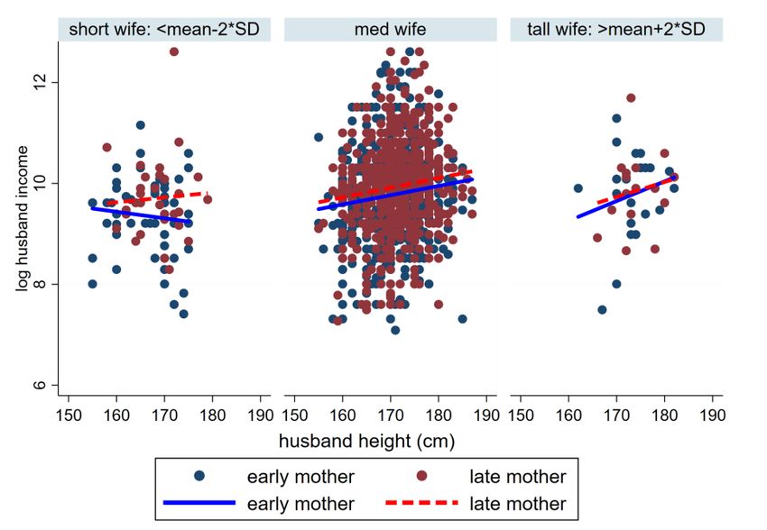
17 / 58

 Again, the WTP between height and income depends on their coefficient at each male profile
height due to the quadratic term. We evaluate the WTP at each of the short (166cm), medium
(172cm), and medium and tall (178 cm) male heights in Table 6.
 [Insert Table 6 here]
 Column (1) shows the WTP of mate-height and mate-income for short women, represented by
the ratio of the percentage change in visits of short women for a one cm increase in male height
over the percentage change in visits for a 1k CNY/month increase in male income. The WTP of
short women (0.457) is higher than that of medium women (0.107) and even tall women (-0.043)
at the height of the short male profile height (166cm). Short women’s (0.109) WTP than that of
medium (0.084) and even tall women (0.053) at the medium male profile height (172cm).
However, at the tall male profile height (178cm), tall women (.149) have the highest WTP,
followed by medium (0.0615) and lastly by short (--.239). The chi2 test shows that the WTP of
short women is significantly higher than that of the medium at the short man’s height, but not at
the medium or the tall man’s height. Short women and tall women are different at the short and
tall men’s heights. Medium and tall women’s WTP are never different from each other. Thus, short
women have the highest WTP of mate-height for mate-income at the short and medium man’s
height, followed by medium women, and then by tall women. However, the opposite ordering is
evident at the tall man’s height. The WTP of each height of woman depends on the man’s height
at which her WTP is evaluated. We find almost identical results when we use the full sample of
1516 female visitors, with the exception of the WTP of the medium woman at the tall men’s height
of 178cm, which becomes insignificant. The change in the WTP across women of different heights
can be summarized by the following observation.
 Observation 3. Women’s WTPs for mate-height forms a U-shaped envelope on the
 women’s height.

 Chinese Family Panel Studies Data

 We test whether these preferences revealed through visits before the first dates in the online
dating environment predict patterns of spousal height in the China Family Panel Studies (CFPS)
2010 baseline dataset. 16 The CFPS is a comprehensive survey of individual-, family-, and

 16
 Although the CFPS for 2012 data is available, it only collected household income without separating husband’s and wife’s incomes.
Moreover, it did not collect the income of self-employed individuals, unlike the 2010 data set.

18 / 58

community-level data across China, covering various aspects of economic and non-economic
issues. It includes 16,000 households in 25 provinces and is representative of the whole population
of China. We restrict the sample to married couples with urban hukous, both between the ages of
20 and 45 years old, which comprises 2191 couples. We drop the observations whose height is
beyond three standard deviations from the mean, which are either outliers or possibly recording
mistakes during the survey. This leaves us a final sample of 2147 couples for analysis. Table 7
shows the summary statistics.
 [Insert Table 7 here]
 Table 8 presents the regressions of the wife’s educational attainment and beauty on husband’s
characteristics. It shows that both the wife’s educational attainment and beauty are positively
related to the husband’s log income and height. We report the ratios and the products of the
coefficients of interest within and across columns in the table. The corresponding Wald test of the
proportionality of these factors is not rejected (p-value = 0.241), indicating that the WTP is
identified. The value of the WTP between husband’s log income and height is between 0.062 and
0.084. This suggests that a one cm increase in height is equivalent to a 6.2-8.4 percent increase in
income for the wife.
 [Insert Table 8 here]
 However, our online dating results suggest that women’s taste for mate-height may be
heterogeneous according to their height. Based on our online dating finding in Observation 3 and
the above subsequent confirmations with marriage data, we predict,
 Hypothesis 4. Short wives are most willing to pay for husband height.

 Heterogeneity in women’s willingness to tradeoff husband income for husband height

 In order to test Hypothesis 4, we apply a methodology recently proposed by Chiappori et al.
(Chiappori et al., 2021). Specifically, assume that men and women are heterogeneous not only in
their observed characteristics, but also in their tastes regarding the characteristics of their potential
spouses. Each woman is characterized by a vector ( , ) ∈ × , where = ( 1 , 2 ) denotes
her observable characteristics (here, education and beauty) whereas = ( 1 , 2 ) denotes her
idiosyncratic preferences for a male’s observable traits. Similarly, each man is characterized by a
vector ( , ) ∈ × , where = ( 1 , 2 ) denotes his income and height while = ( 1 , 2 )

19 / 58

summarizes his tastes regarding the education and beauty of a potential mate. The surplus
generated by the matching of WTP. ( , ) and Mr. ( , ) takes the form:
 ( , ; , )=( , )+∑ +∑ Eq. (2)
where ( , ) is a systematic component reflecting the overall interaction between the spouses’
observable characteristics, while the next two terms translate each spouse’s idiosyncratic
evaluation of the partner’s traits.
 In practice, we assume that the vectors of random variables ε and η are independent of each
other and of observables, and normally distributed with mean 0 and variance 1. Similarly, x is
normally distributed, with mean Mx and covariance matrix Σxx, while y is normally distributed,
with mean My and covariance matrix Σyy. Finally, the surplus is assumed quadratic:
 ( , ) = ′ ∆ Eq. (3)
 Under these assumptions, Chiappori, McCann, and Pass (2021) show the following results.
First, the joint distribution of (x, y) at the stable matching is normal. Second, the structure just
described implies the following two relationships between x and y:
 = + + Σ Eq. (4)
and
 = + + Σ Eq. (5)
A, B, Σx and Σy are 2 x 2 matrices; moreover, it is then the case that
 ∆= ′ (Σ )−1 + (Σ )−1 Eq. (6)
where ′ is the transpose of A.
 lt follows from these results that the matrix ∆ can readily be estimated. Indeed, in equation (3)
the random term Σxη is independent (by assumption) from the regressor, and can, therefore, be
estimated by OLS; in practice, one must simply regress the wife’s characteristics over the
husband’s to identify the regressors A and the covariance matrix Σx. Similarly, regressing the
husband’s characteristics over the wife’s gives matrices C and Σy.
 Finally, a particular case obtains in the index case, studied by Chiappori et al. (Chiappori et
al., 2012), when the vectors of observable characteristics x and y enter the surplus through one-
dimensional indices I(x) and J(y) respectively. In the linear case under consideration, we then
have:
 ( ) = ′ , ( ) = ′ Eq. (7)

20 / 58

where α and β are vectors in . It follows, in particular, that both matrices A and C are of rank
one, a property that can readily be tested.
 We divide our data into three subsamples based on the wife’s height: short (one standard
deviation below the mean height), medium, and tall (one standard deviation above the mean
height), and then run Eq. (4) separately on these three subsamples to obtain the corresponding
WTP for each type of wife. By comparing the values of their WTPs between husband height and
husband income, we can identify which type of wife values the height of their husband most.
 However, differences in the measured WTPs of wives for husband height across groups may
be due to their husband’s preferences, not the wife’s preferences. In this case, the assumption of
Chiappori et al. (Chiappori et al., 2021) that the unobserved characteristics of husbands are not
correlated with their observable characteristics may be violated when we divide wives into short,
medium, and tall groups. To address this problem, we apply the estimator that Vella (Vella, 1993)
developed to adjust for the possibility of unobserved selection with simultaneous equations. We
use the wife’s mother’s age of giving birth and the wife’s weight at birth as exclusion restrictions
for the wife’s height and to run the first-stage regression in Table 9.
 [Insert Table 9 here]
 We expect that mother’s age of giving birth is positively correlated with children’s height,
because the resources available to the child, which increases with the mother’s age, contributes to
realized adult height. Older mothers are more knowledgeable than younger ones. Such
knowledgeability has been shown to contribute to the height of children (Rubalcava & Teruel,
2004; Thomas, Strauss, Henriques, Strauss, & Henriques, 1991) through better utilization of
community and household resources, and possibly by improving child nutrition (Bhargava & Fox-
Kean, 2003). By contrast, the mother’s age should not be correlated with the traits related to marital
matching of the daughter, including her beauty.
 Potential height and beauty (e.g., symmetry of facial features and body proportion) are
influenced by genetic quality, prenatal hormonal levels, and exposure to diseases and parasites
(Gangestad, 1993; Richard H. Steckel, 2009). Qualitatively, physical beauty is generally related to
averageness, symmetry, and sexual dimorphism of features (Rhodes, 2006). In women, beauty is
also a signal of fertility, e.g., levels of estrogen. For beauty, genes, mutation, a parasitic load plays
the dominant role, rather than resources (Gangestad, 1993). Thus, the father’s age can decrease his
child’s beauty because men produce new sperm throughout their lives. Sperm produced at later