Measuring subnational economic complexity: An application with Spanish data - JRC Working Papers on Territorial Modelling and Analysis No 05/2019 ...

Measuring subnational economic
complexity:

An application with Spanish data
 JRC Working Papers on
 Territorial Modelling and
 Analysis No 05/2019

 Pérez-Balsalobre, S., Llano-Verduras, C.,
 Díaz-Lanchas, J.

 2019

This publication is a Technical report by the Joint Research Centre (JRC), the European Commission’s science
and knowledge service. It aims to provide evidence-based scientific support to the European policymaking
process. The scientific output expressed does not imply a policy position of the European Commission. Neither
the European Commission nor any person acting on behalf of the Commission is responsible for the use that
might be made of this publication.

Contact information
Simone Salotti
Edificio Expo, c/Inca Garcilaso 3, 41092 Sevilla (Spain)
Email: jrc-b3-secretariat@ec.europa.eu
Tel.: +34 954488463

EU Science Hub
https://ec.europa.eu/jrc

JRC116253

 PDF ISSN 1831-9408

Seville: European Commission, 2019

The reuse policy of the European Commission is implemented by Commission Decision 2011/833/EU of 12
December 2011 on the reuse of Commission documents (OJ L 330, 14.12.2011, p. 39). Reuse is authorised,
provided the source of the document is acknowledged and its original meaning or message is not distorted. The
European Commission shall not be liable for any consequence stemming from the reuse. For any use or
reproduction of photos or other material that is not owned by the EU, permission must be sought directly from
the copyright holders.

All content © European Union, 2019

How to cite this report: Pérez-Balsalobre, S., Llano-Verduras, C., and Díaz-Lanchas, J. (2019). Measuring
subnational economic complexity: An application with Spanish data, JRC Working Papers on Territorial Modelling
and Analysis No. 05/2019, European Commission, Seville, JRC116253.

The JRC Working Papers on Territorial Modelling and Analysis are published under the editorial
supervision of Simone Salotti and Andrea Conte of JRC Seville, European Commission. This series addresses the
economic analysis related to the regional and territorial policies carried out in the European Union. The Working
Papers of the series are mainly targeted to policy analysts and to the academic community and are to be
considered as early-stage scientific articles containing relevant policy implications. They are meant to
communicate to a broad audience preliminary research findings and to generate a debate and attract feedback
for further improvements.

Acknowledgements
This paper was developed in the context of two research projects: The C-intereg Project
(www.c-intereg.es) and ECO2016-79650-P from the Spanish Ministry of Economics and
Innovation. We are grateful for the suggestions received during the international
workshop on Economic Geography organized in Utrecht University and the GeoInno2018
in Barcelona. Jorge Díaz-Lanchas also wants to thank CID Harvard for receiving him as a
postdoctoral visiting scholar during the Fall 2016, when the embryo of this article started
to grow. We also want to thank additional comments received in the ETSG-2017 and the
2018 RSA-Smarter Conference on Territorial Development, as well as insightful remarks
from Asier Minondo and Rocío Marco on previous version of this manuscript. We finally
thank Pedro Rodriguez for his valuable language help.

Abstract
Economic complexity indicators provide a better understanding of the long-term
determinants of countries’ economic growth. However, they do not account for intra-
national spatial heterogeneity, even when regions, and not only countries, differ
tremendously in their productivity. This paper tries to fill this gap by developing a
methodology to estimate economic complexity at the subnational level using a unique
trade database on intra-national trade flows for Spain. Specifically, we calculate
international and intra-national economic complexity indicators for the provinces of Spain
(NUTS-3) for the period running from 1995 to 2016. We find that regions tend to differ in
complexity not only in time but also in their international and intra-national trade
exposures. We also show that indicators that incorporate both types of trade flows are
better predictors of future GDP growth. These findings shed light on the determinants of
regional convergence patterns.

Measuring subnational economic complexity:
 An application with Spanish data

 Santiago Pérez-Balsalobrea,b, Carlos Llano-Verdurasa,b, Jorge Díaz-Lanchasc
 a
 Autonomous University of Madrid
 b
 L.R. Klein Institute
 c
 European Commission, Joint Research Centre

JEL: R11, F1, O4.

1. Introduction

The accumulation and diffusion of knowledge are key drivers of long-term economic
growth (Lucas, 1988). Even when the theoretical underpinnings are clear, the
question of how to measure empirically knowledge creation remains open. Several
approaches and data sources have been used for the measurement of knowledge
creation including number of patents (Boschma, et al., 2014; Balland and Rigby,
2016), migration flows (Andersen et al., 2011), investment flows (OECD, 2013),
and international trade flows (Hausmann and Hidalgo, 2011).1 Concretely,
Hausmann and Hidalgo (2009, 2011, 2014) improved upon the concept of economic
complexity (EC from now onwards) and defined a national indicator that could
measure the non-observable capabilities (know-how) embedded in the production
of goods and services. This indicator is calculated through an iterative process
between a country’s diversification (the number of products that a country exports
with revealed comparative advantage) and a product’s ubiquity (the number of
countries with revealed comparative advantage in that product). That is, countries
with more capabilities can make more products (higher diversification), whereas
products that also require more capabilities to be produced are accessible to fewer
countries (lower ubiquity).
This points out to a positive relation between a country's capabilities and its future
economic growth. Yet these capabilities may not be evenly distributed throughout a
country's space or may even be concentrated over short distances: for example,
cities (Díaz-Lanchas, et al., 2017). This is the starting point of our analysis. We
resort to intra-national trade data and compute a complexity indicator for each
Spanish subnational entity, attending to both its international and its intra-national
trade dimensions. Specifically, we cover the 50 Spanish provinces (NUTS-3, in
Eurostat terminology) with a 29-product disaggregation for the period 1995–2016.
In line with previous research (Reynolds et al., 2017; Gao and Zhou, 2018), our
contribution relies on the combination of inter and intra-national trade flows for
each province and product, bridging the gap between the (desired and usually
unobservable) intra-national complexity and the international one.2
Our goal is to contribute to the literature of economic complexity and regional
science by taking a closer look at the spatial dimension. Provinces (NUTS-3) are
good proxies for actual production locations and, therefore, amenable to the

1
 See Corrado and Hulten (2010) for an in-depth review.
2
 As stated in previous research (Hausmann et al., 2014), the empirical measurement of knowledge
 creation should be based on production data but is instead mainly based on international trade data,
 because of the latter's highly standardized and disaggregated features for most countries.

economic complexity framework. Besides, they are more comparable spatial units
than regions (NUTS-2) in both size and geographic characteristics. Indeed, they are
the most comparable spatial units to cities, for which trade data are not officially
available neither estimated. This fine spatial scale and great trade granularity allow
us to explore the heterogeneity across regions and sectors within countries, and to
show thereby that only international trade-based complexity indicators lead to
biased estimations of the computed indicators when spatial heterogeneous patterns
are not accounted for.
Our estimation of subnational indicators begins with the complexity indicators
provided by the Atlas of Economic Complexity (2011). Our data on international
trade flows come from the official Border Custom database and have a high level of
product disaggregation. For the interregional dimension, we draw from a unique
database of intra-national flows for Spain (Llano et al., 2010) that enables us to
categorise intra-national trade flows into interprovincial and intra-provincial
bilateral flows, with disaggregation into 29 sectors for Spain. Both databases are
compiled for the same time series (1995–2016) and represent a first attempt to
merge two trade databases of different natures at a fine spatial level with the
complexity indicators. Therefore, we believe that our analysis is a promising effort
to estimate economic complexity indicators at the subnational level in Spain while
taking into account both international and interregional dimensions.
An important limitation that arises when extending the approach in Hausmann and
Hidalgo (2009) to subnational entities is the conceptual leap from production data
to international trade data. First, trade intensity is higher within national boundaries
due to the trade impediments posed by international borders (Álvarez et al., 2013;
Gallego and Llano 2017). For instance, around 82% of the Spanish economy's total
trade remains within national boundaries. 3 Moreover, there is great spatial and
sectorial variability in the share of international exports within countries, which may
bias any complexity index not accounting for such spatial and sectorial
heterogeneity.
To overcome these limitations, we use two different methodologies to estimate the
economic complexity indices at the province level, and then compare and test the
results. We expect these methodologies to shed light on at least three dimensions.
First, they should allow us to see how the complexity framework is enriched when
we incorporate intra-national trade into international flows. Second, they should
help us understand the relationship between economic complexity indicators
computed from international and intra-national flows for subnational entities and
the consistent bias towards high-complex products. Our hypothesis is that the
economic complexity computed for international flows should be higher than that
for intra-national flows. This intuition is based on the trade literature on
heterogeneous firms (Melitz, 2003; Melitz and Treffler, 2012; Melitz and Redding,
2014), according to which only the most productive firms can overcome the fixed
costs of exporting, and on quality patterns (Hummels and Skiba, 2004; Hummels
and Klenow, 2005) that emphasize the role of exporters in trading high-quality
products overseas. Third, our methodology helps us to assess the appropriateness
of our intra-national complexity indicator vis-à-vis the international one. That is, we
try to determine whether international complexity or subnational interregional
complexity is the more prominent indicator of future provincial GDP per capita.
According to the results, our indicator containing all types of trade flows provides a
better fit and has better predictive properties than an indicator that takes only
international trade flows into account.
The remainder of the paper is organised as follows. Section 2 reviews previous
works on regional complexity indicators to better frame the main contribution of our
paper. Section 3 describes our methodology, and Section 4 does the same for data.

3
 Own calculation from the C-intereg project, as explained below.

Section 5 contains the descriptive analysis and an econometric analysis of our
indicators' validity. Section 6 concludes with a set of policy implications.

2. Theoretical framework

It is difficult to compute subnational trade-based EC indices because there are no
official intra-national trade databases. Previous works have recently tried to get
around this problem resorting to different and complementary databases. Reynolds
et al. (2017) generated a rich dataset of EC indices for Australian subnational
entities by drawing from a novel trade database of multi-regional Input-Output (IO)
tables, with nine regions and 506 sectors. The authors isolated trade flows among
Australian regions and between those regions and the rest of the world. Such work
built upon previous research by Wood and Lenzen (2009) who provided a first
estimate of EC indices using IO data from 1975 to 1999 for 344 intermediate
industry sectors. However, they dealt only with national economic structures,
whereas Reynolds et al. (2017) applied Hausmann and Hidalgo's EC concept
(Hausmann et al., 2014; Hidalgo & Hausmann, 2009) to Australia’s interstate and
international exports, finding that small differences in industrial capabilities were
crucial for relative measures of complexity. Concretely, they found that most
Australian states (especially in Western Australia) were exporting primarily
resource-intensive goods, whereas interstate trade mainly specialized in complex
products that are not internationally exported.
Gao and Zhou (2018) estimated the EC of Chinese provinces for 1990–2015. Their
work is novel in its use of firm-level data and allows them to consider both
international and intra-national trade flows for goods and services. Their analysis
points out potential problems in the calculation of EC indices with world trade data
exclusive of industries that do not export abroad. They find that the EC ranking of
Chinese provinces was stable over time, with coastal provinces having higher EC,
but also that diversified Chinese provinces tended to have less ubiquitous
industries.
Finally, Balland and Rigby (2016) offered an interesting analysis of subnational EC
measures for the US. In contrast to the above articles, they addressed the spatial
distribution and the change in complexity of US cities using an extensive patent
database from the US Patent and Trademark Office. Identifying the technological
structure of US metropolitan areas from 1975 to 2010, they found that knowledge
complexity had an uneven spatial distribution among US cities. They also tested the
spatial diffusion of knowledge to assess whether it was linked to complexity levels,
finding that complex technologies were less likely to be located in remote cities. On
the contrary, they found a high concentration of highly complex activities in a few
productive locations.
This is not an exhaustive account, but these works have laid out the theoretical and
empirical groundwork for our paper. We go beyond an analysis with IO tables to
use Spain's international and intra-national bilateral trade flows at the smallest
possible spatial units up to the present. We believe that controlling for these two
types of (tradable) flows for 50 subnational entities and 29 sectors allows us to
compute complexity indicators considering products' destination markets
(international or intra-national) and accounting for biases in the computation of EC
indicators. Moreover, we believe we can approximate complexity patterns over
short distances (almost at the city level) and assess economic performance for
these precise spatial locations.

3. Methodology for the estimation of subnational economic complexity
We take two approaches to build a subnational economic complexity indicator. In
the main text we focus on our baseline indicator, leaving our second approach to
Annex A.1.

 3.1.Baseline approach

Our baseline approach relies on the estimation of EC indicators (ECIs) at the
subnational NUTS-3 level (provinces) in Spain by matching product complexity
indicator (PCIs) for international flows at the country level with our two trade
databases at the province level.4 In this way we assume that a given product has
the same level of complexity—i.e. skills embedded in its production—regardless of
the location (or market) where the product is actually produced.
Prior to this, we calculate the region's comparative advantages (RCAs) in every
product (or sector)5, for international, intra-national and total trade flows. These
RCAs are compiled into a matrix (M) in the following form:

 ∑ 
 
 = / (1)
 ∑ ∑ 

where refers to the exports of a certain product or sector (s) in a given region
(r) at time (t) for each type of trade flow (F). Matrix M is similar in structure to the
matrix in Hausmann and Hidalgo (2009), taking the value 1 when RCA>1 and 0
otherwise.
The nature of our trade dataset leads us to calculate different ECIs for each
province using different trade flows. In the case of international trade, there is a
direct and equivalent product classification between the PCIs obtained by
Hausmann and Hidalgo (2011) (at HS4 product classification) and our subnational
international exports (from Border Customs).

A problem arises when merging international PCIs with intra-national trade flows.
The latter flows use a different product classification, because of the different data
sources used for their compilation. As a result, we need to match the international
PCIs to a product classification that is similar in both the intra-national trade flows
and the international PCIs. Then, we can aggregate the latter into an intra-national
PCI consistent with our sectorial classification.6 More specifically, we calculate an
equivalent PCI for each sector and region using international trade flows according
to the following:

 ∑ 
 
 = (2)
 ∑ 

4
 Available at http://atlas.cid.harvard.edu/.
5
 Throughout the analysis the two terms are used interchangeably
6
 This sectorial classification is shown in Annex 2. We pursue three methods of aggregation: simple
 averages, weights using quantity flows (tons) and monetary flows (euros). We then test the
 performance of the three PCIs and ECIs obtained, and consider the weights in euros as the most
 appropriate.

where stands for the HS4 PCIs obtained by Hausmann and Hidalgo (2011)
 
and stands for the HS4 international exports. Note also that is
determined by the international product-mix in a given region's trade basket.
 
With , we can now recalculate our final PCI with the following expression:

 ∑ 
 = 
 (3)
 ∑ 

where, again, F refers to each type of trade flow. Thanks to , we can estimate
the EC indicator for each region:

 ∑ 
 
 = (4)
 ∑ 

With expression (4), we estimate an ECI for international and intra-national flows.
Additionally, as explained in the next section, our intra-national trade flows can be
split into interregional trade flows (province to province) and intraregional flows
(within the same province). Taking this advantage in granularity, we exploit the
spatial heterogeneity of our subnational ECI and create two additional indicators:
 
 and . This way, we come up with smaller (intraregional)
indicators.
Finally, we develop an ECI for total trade flows regardless of destination market. To
this end, we first aggregate international trade flows for Spanish provinces to the
 
equivalent intra-national sectorial classification. Then we recalculate the RCAs ( )
 
in Equation (1) to get the PCIs using expression (3) and finally an indicator
according to (4).

4. Data
Our dataset includes both international and interregional trade flows at the NUTS-3
level. The international trade flows correspond to the official records published
annually by the Spanish Tax Agency (AEAT) 7 for each Spanish province. The value
of this type of data lies in its great product disaggregation (CN8-digits product
classification). We collected data from 1995 to 2016 and compiled a database of
around 38 million observations. We then matched the CN8-digits product
classification with the HS4 product classification used by the PCI database (around
1,240 products per year) and aggregated the CN8-digits products to HS4 products
with their corresponding complexity levels, weighted by monetary values.
The intra-national trade flows database is based on the C-intereg database,8 first
compiled by Llano et al. (2010) and updated annually until 2016. This database
includes bilateral trade flows between the 50 Spanish provinces at the NUTS-3
level, covering a long period of time (1995–2016). The compilers of the C-intereg
database took the official data on bilateral flows by transport mode (road, railway,
ship and aircraft) and then matched these flows with the official data on production
and international exports, filtering by re-exporting flows at the province and
sectorial levels for each year in the period 1995–2016. The result was a panel
database with around 25 million observations encompassing all 50 provinces and 29
7
 Data available at the Border Customs and Spanish Tax Agency (www.aeat.es).
8
 Available at http://www.c-intereg.es/.

sectors. As reported in previous papers mixing this database with the official
international trade flows for Spain, the range of products and destinations is wider
here than it is for international flows (Diaz-Lanchas et al., 2019). Table 1
summarizes the spatial and sectorial disaggregation of both databases.

 Table 1: Summary of trade data used
 Territorial Initial product
 Trade flow Time period Source
 Disaggregation disaggregation
 International NUTS-3 More than 10000 1995-2016 AEAT
 Intra-national NUTS-3 29 1995-2016 C-intereg

Finally, for the econometric analysis, we complemented our panel database with
NUTS-3 variables corresponding to factor endowments. Specifically, we included the
(net) physical capital (PC) and the (economic value of) human capital (HC) for each
region (province) in the period 1995–2013. Both variables are taken from Instituto
de Investigaciones Valencianas (IVIE) 9 and are used in Section 5.

5. Results

 5.1.Descriptive Analysis
First, we check the stability over time of the international trade structure. Figure 1
represents the share of international exports over total exports in 1995 and 2016
for each Spanish province. In line with Gao and Zhou (2018), the results clearly
point to a stable trade structure but also, and differently from them, to a
dichotomic internationalization of Spanish provinces. The shares of international
exports of some provinces increase from 18% in 1995 to more than 27% in 2016,
whereas half the provinces have below average values throughout the whole
sample period. Recent evidence (Requena and Llano, 2010; Llano et al., 2017;
Díaz-Lanchas et al., 2019) suggests that these differences in spatial
internationalization result not only from differences in knowledge creation, but also
from location determinants. This means that there's a tendency of firms within a
country to select their location considering both the conditions of the local labour
markets (factor endowments) and transport costs. Location determinants dictate
the transport mode used as well as the average distance of each flow. Coastal
locations have a comparative advantage in trading heavy products, such as
minerals, iron-steel and windmill components, whereas internal regions specialize in
other tradable products (Gallego et al., 2015).

9
 Available at https://www.ivie.es/.

Figure 1: Change in share of international exports by province: 1995 vs
2016

Source: Own elaboration with C-intereg and AEAT data.

This stability in trade structures also holds when looking at the products' data.
Figure 2 shows the share of international exports over total exports for each of the
29 sectors in 1995 and 2016. Again, the results suggest that more than half of the
sectors are oriented towards the internal rather than the international market. Only
six out of 29 sectors have more than 50% of their production geared towards
international markets. Four of these are high-complex sectors (electric and non-
electric machinery, transport equipment and furniture and other goods), whereas
the other two are low-complex sectors (leather and footwear and food oil). Because
of the spatial and sectorial trade structures in such cases, and their orientation
chiefly towards internal national markets, the computation of ECI can result in
biased indicators. We can therefore enrich our estimation of know-how in the
regional production of these products by considering intra-national trade flows
jointly with international flows, where only some (special) products are exported.

Figure 2: Change in share of international exports by product (R30).
 1995 vs 2016.

Note: The size of the bubbles represents the sector’s complexity in 1995.
Source: Own elaboration with C-intereg and AEAT data.

To further illustrate intra-national trade characteristics, Figure 3 plots the
relationship between product complexity and the average distance travelled by
product for all types of trade flows. The size of each bubble represents a product's
total exports. It is easy to distinguish two groups of products. Those in grey, such
as oil (food), correspond to low-complex products travelling long distances (more
than the maximum average distance for intra-national trade flows). But there are
also low-complexity products travelling mostly short distances, which points to an
overconcentration of such trade flows within the country (the minimum and median
average distance for inter-regional trade are 210 km and 400 km respectively). The
second group, in blue, shows a positive relationship between trade intensity and
distance. First, a number of low-complex products (cement; rocks, sand and salt;
cereals; fertilizers; tobacco; wood; live animals) are associated with trade
intensities over short distances. These are products traded mainly among Spanish
provinces (and regions). We also observe trade flows in middle distances for
products of average complexity (processed food), corresponding to large
interregional flows (e.g. Cataluña–Andalucía–C. Valenciana–Madrid) and short
international ones (Spain–EU countries). Finally, other sectors such as chemical
products, machinery (electric and non-electric) and transport equipment, are
characterised by high complexity and long-travel distances. Their share of
international exports is the greatest. The pattern plotted in Figure 3 points to an
overrepresentation of high-complex products in international trade statistics.
The previous patterns clearly point to heterogeneous spatial trade patterns;
therefore, we should expect spatial differences in the ECI. In Figure 4, we split the

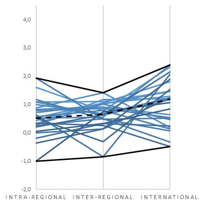
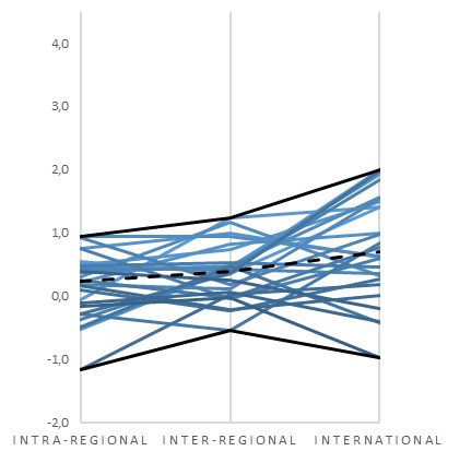
sample of 50 Spanish provinces into three groups according to their EC and using
 
the indicator in 2016. The results for the beginning of the period (1995) are
shown in Figure A.3 in Annex 3. The first group contains provinces in the first
quartile (the 12 provinces with the lowest complexity); the second group contains
provinces in second and third quantiles (26 mid-complexity provinces); and the
third group is made by provinces in the fourth quantile (the 12 with the highest
complexity). Additionally, each group is subdivided by the three EC indicators (for
intraregional, interregional and international economic complexity) explained in
Section 3.1. Panels A to C represent the trade structures for each group of
provinces, with the median, minimum and maximum level of complexity added in
for each trade typology, whereas the map in Panel D shows the geographic
distribution of the total EC indicator.
Several points are worth mentioning here. Panels A to C highlight the positive
relation between a product's economic complexity and the destination market,
being the complexity higher the further the market (e.g. international destinations).
Also interesting is the geographic distribution of complexity (Panel D). The most
complex regions are the ones with the largest Spanish cities (Madrid, Barcelona and
Valencia) and the ones hosting either innovation hubs (País Vasco and Navarra) or
even complex industries such as the automotive sector (Valladolid, Palencia,
Zaragoza and Pontevedra).10

10
 In Annex 3, Figure A.3 shows the results for 1995. It highlights the spatial stability of EC indicators in
 time. There are only a few changes, mainly in the low-complexity group. In comparison with Figure 4
 for 2016, EC indicators for 1995 point to higher levels of complexity, consistent with the recent decay
 in Spain's ECI published by the Atlas of Economic Complexity. Also note the higher complexity of the
 provinces (Guadalajara) surrounding provinces with big cities inside such as Madrid as a result of the
 agglomeration economies’ effects of the latter.

Figure 3: PCI (with total trade) and average distance travelled. 2016.

Note: The size of the bubbles represents the total trade of the sector (in €). The dotted line represents
the maximum average distance travelled by intra-national trade flows (812 km).
Source: Own elaboration.

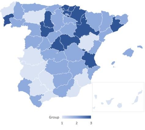
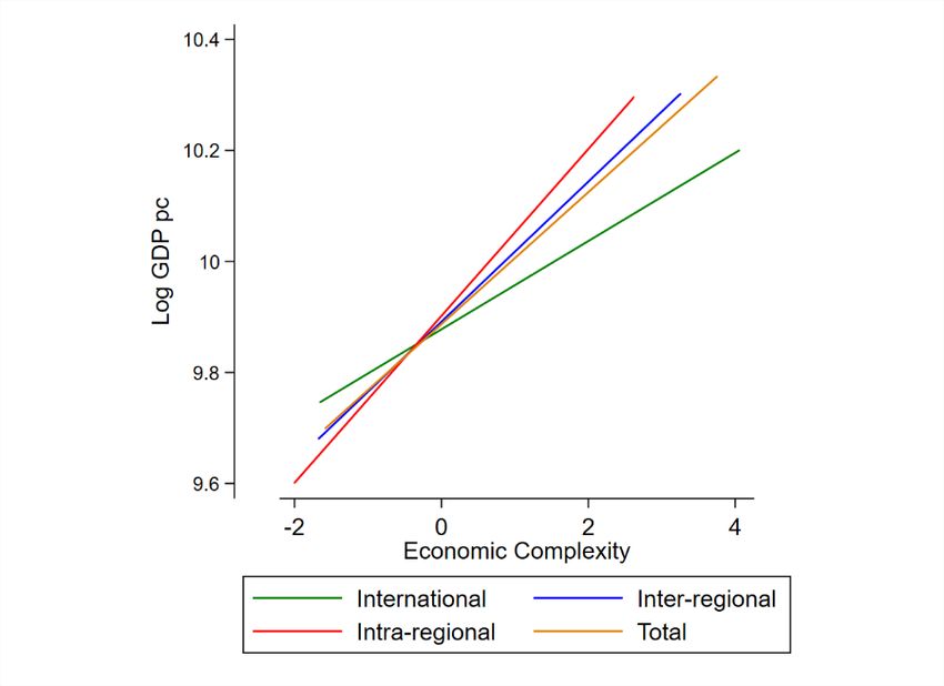
Figure 4: ECI by region and trade flow (2016)

 Panel A: Low-complex regions Panel B: Middle-complex regions

 Panel C: High-complex regions Panel D: Total ECI by regions

Panels A-C: Each colour bar belongs to a province (Nuts 3). Black lines refer to minimum and maximum
complexity in each represented trade flow. The dotted line indicates the median of each group.

Panel D: Group 1 refers to low-complexity regions (first quartile), group 2 refers to mid-complexity
regions (second and third quartiles) and group 3 to high-complexity regions (fourth quartile).
Source: Own elaboration.

The use of multiple ECI raises the question of their explanatory power. Figure 5
shows the relationship between GDP per capita (GDPpc) and the four ECI. While all
indicators are strongly and positively related to GDPpc, the relationship is weaker
for the ECI calculated only with international trade flows (this is particularly evident
for high levels of EC). On the other hand, the total ECI with both international and
intra-national trade flows provides a better explanation of GDPpc.

Figure 5: GDP per capita vs ECI at the province level (baseline approach)

Source: Own elaboration.

Figure 6 shows the R-squared obtained when regressing GDPpc ten years forward
(including the whole sample) with each of the four EC indicators separately
(detailed results not reported for the sake of brevity, but available upon request).
We also estimate two additional versions of the model adding controls for factor
endowments: namely, HC and PC, as drivers of GDP per capita. The results show
that all variables have a positive and significant relation with future GDPpc. Figure 6
reinforces our hypothesis that intra-national trade flows are even more important
than international trade flows in explaining future GDPpc. Indeed, the EC indicator
for total trade flows provides outstanding results, explaining almost 40% of future
GDPpc. For the provinces with zero or small share of international trade flows (as
evidenced in Figure 1 for half of the provinces), intra-national EC indicators gain
huge explanatory power. Finally, note that all the models including ECI report even
larger R-squared than the models including standard variables in the literature
(orange bars).

Figure 6: R-squared GDP per capita (t+10) and EC indicators
 (baseline approach)

Source: Own elaboration.

Even when the ECI obtained fit well with future (provincial) GDPpc, these regional
indicators can also be affected by the country’s specific dynamics. When a country
such as Spain reduces its complexity with respect to the rest of the world, then it is
reasonable to think that its regions (provinces) will undergo an equivalent process.
To investigate this possibility, Figure 7 plots the Spanish GDPpc, the total ECI
computed, and the classical regional economic growth factors (PC and HC) per
capita. GDPpc is presented as a ratio of world GDPpc to assess whether relative
changes in the Spanish economy have been accompanied with vis-à-vis changes in
the world economy. Panel A shows the evolution of the Spanish GDPpc (red line)
and its ratio in the world's GDPpc (dotted blue line). Both variables show a clear fall
from 2008 to 2012, which becomes even more abrupt in the case of GDPpc relative
to the world. Panels B-D compare this relative ratio with the ECI (Panel B), the
physical capital (Panel C) and Human Capital (Panel D). As observed, the ECI is the
variable that most clearly mirrors the dynamics of the Spanish GDPpc relative to
the world's GDPpc. PC shows a monotonic growth path, whereas HC presents
changes peaks and rebounds similar to GDPpc but some years in advance to the
latter. These dynamics are coherent with the striking pattern of the Spanish
economy by which it has drastically reduced its economic complexity in comparison
to the rest of the world since the beginning of the crisis. Last, Figure 7 again
emphasizes the explanatory features of the total EC index in detriment of its PC and
HC counterparts.

Figure 7: Evolution of the Spanish GDPpc, the regional ECI and regional
 economic factors per capita (physical and human capitals). 1995-2016.

 Panel A: GDP per capita Panel B: Total Economic Complexity

 Panel C: Human capital per capita Panel D: Physical capital per capita

Note: Blue (dotted) lines represent Spanish GDP per capita over world GDP per capita. The red line
represents Spanish GDP per capita. The orange line represents Spanish total economic complexity.
The green line represents Spanish human capital per capita. The black line represents Spanish net
capital per capita. All variables are in real terms.

Source: Own elaboration.

 5.2.Econometric Analysis
The previous section was devoted to the illustration of the main features of the EC
indices calculated with the Spanish data. This section deals with the econometric
analysis aiming to explain future growth of income per capita. As previously stated,
our specifications also include two variables widely discussed in the literature: PC
and HC both in per capita terms. Thus, our two main specifications take the
following form:

( / ) +5 = 1 + 2 + 3 + + (5)
( ) +5 = 1 + 2 + 3 + + (6)

Where GDPpc refers to provincial GDP per capita, does the same with world
GDP per capita and controls with time-fixed effect. Note that equation (5)
assesses the impacts of the ECI over the 5-years growth of a relative measure of

(world) GDP, whereas equation (6) does the same with the 5-years growth of the
 absolute value of provincial GDP.11
 Table 2 contains the results for equations (5) and (6) in a cross-section between
 the initial and the last year for each five-years period using OLS estimators with a
 year fixed effect for the last year. The main model (M1) refers to the complete
 specification with the ECI (considering total trade flows) and the PC and HC
 variables as regressors. In Models M2-M4 we combine different specifications
 dropping variables correspondingly. The last line of the table shows the change in
 R2 over the main specification (M1) as a measure of the performance of our models.

 Table 2: GDP per capita growth (t+5) by province. Baseline specifications.
 Cross-sections between the first and the last year every t+5 years. OLS
 estimators.

Years-
 1995-2000, 2000-2005, 2005-2010, 2010-2015
Thresholds

 M1 M2 M3 M4 M1 M2 M3 M4

Year FE YES YES YES YES YES YES YES YES

VARIABLES GDPpc/World GDPpc (t+5) GDPpc (t+5)

Total ECI 0.393*** 0.395*** 0.437*** 0.316*** 0.318*** 0.398***
 (0.0528) (0.0581) (0.0556) (0.0460) (0.0541) (0.0533)
Physical cap. 0.317*** 0.320*** 0.369*** 0.376*** 0.378*** 0.474***
 (0.0784) (0.0861) (0.0571) (0.0728) (0.0774) (0.0557)
Human cap. 0.117 0.317*** 0.277*** 0.219*** 0.379*** 0.408***
 (0.0827) (0.0886) (0.0604) (0.0769) (0.0809) (0.0560)

Observations 200 200 200 200 200 200 200 200
R-squared 0.551 0.425 0.483 0.543 0.603 0.518 0.503 0.573

Change in
 22.90% 12.30% 1.50% 14.10% 16.58% 4.98%
R-squared

Robust standard errors in parentheses
*** p

database (Tables A.4.3 and A.4.4). The EC indicators are always associated with
positive and significant coefficients, and their impact appears to be even higher the
longer the time period considered.

Figure 8 summarizes this information. Specifically, we show the change in the R 2
for different years-thresholds (5, 10, 15 years) when explaining (provincial) GDPpc.
For shorter periods (5 years), PC appears to have a good explanatory power,
particularly for the growth of absolute GDPpc. Nevertheless, EC becomes the only
one variable capable of accounting for the largest proportion of provincial GDPpc (in
relative or absolute values) in 10 and 15 years-periods. Thereby, we highlight the
total EC index as clearly the most relevant variable explaining future long-run
regional economic growth.

 Figure 8: R2 changes in explaining provincial (relative and absolute) GDP
 growth rates.

 Panel A: GDPpc over world GDPpc Panel B: GDP per capita

Source: Own elaboration.

Finally, Table A.4.5 (in the Annex 4) differentiates by the international, inter-
regional and intra-regional EC indicators. The results are robust and consistent with
those in Table 2, and confirm the higher impact of the international EC indicator
over its intra-national counterparts, as argued in the descriptive analysis. This
reinforces our hypotheses on the higher complexity levels of international trade
flows, pointing out to an over-representation of complex products in international
statistics. All these results allow us to conclude that ECI are key in explaining future
GDPpc growth once we control for different factor endowments, in line with
previous works (Hausmann and Hidalgo, 2009, 2011 and 2014). Nevertheless, our
results give evidence on the biases introduced when using only international trade
statistics. These problems are solved when adding intra-national trade flows in our
analysis.

6. Conclusions
Knowledge is unevenly distributed in space. Up to now, several attempts measuring
the concept of EC rely on country-level analysis using international trade statistics,
even when the highest share of economic activity remains within national borders
and present humongous heterogeneity across regions and places. This scarcity in
intra-national analysis is due, at least partly, to the scarcity of publicly available
subnational data.

In this paper we propose a novel approach to compute subnational ECIs for the
case of Spain and its 50 provinces for the period 1995–2016. Our main
methodological contribution entails the combination of international and intra-
national trade flows statistics as well as economic complexity indicators. To the best
of our knowledge, our analysis is the first attempt to estimate economic complexity
indicators at the subnational level in Europe with bilateral trade data.

Thanks to this effort, we elaborate a new set of economic complexity indicators that
allows us to account for cross-regional differences in income per capita. Our results
reinforce the importance of economic complexity as a leading indicator of future
GDP per capita. We also confirm that economic complexity is enriched by the
inclusion of intra-national trade flows. Indeed, we show that economic complexity
indicators based only in international trade statistics are usually biased towards
most complex products. We also show a positive relation between complexity and
the average distance of trade flows, and find that total EC indices outperform those
that only consider international trade flows, especially in the very long run.

Our results entail interesting indications for future economic policies. One of the
great problems in current economic policy is to determine at which level of
territorial disaggregation we should apply political and economic measures for
maximum efficacy. Most researchers consider cities and metropolitan areas to be
the new nations. The methodology we propose reflects this notion and focuses on
the lowest territorial disaggregation possible. This helps us to develop clever
strategies to optimise the sectoral structures of lagging regions, making them more
resilient and boosting their capacity to succeed in a more global economy. We
expect to shed new and prominent light on this relation in future research, going
deeper in the dynamics of those regions that seek both to penetrate the farthest
markets (first within their country, then in the rest of the world) and to produce
more innovative and competitive products.

7. References
Alvarez, F.E., Buera, F.J., Lucas, R.E., Jr., 2013. Idea Flows, Economic Growth, and
Trade. NBER Working Paper Series w19667.

Andersen, T.B., Dalgaard, C., 2011. Flows of people, flows of ideas, and the
inequality of nations. Journal of economic growth 16, 1-32.

Balland, P.A., Rigby, D., 2017. The Geography of Complex Knowledge. Economic
Geography 93, 1-23.

Balland, P.A., Jara-Figueroa, C., Petralia, S., Steijn, M., Rigby, D., and Hidalgo, C.,
2018 Complex Economic Activities Concentrate in Large Cities. Papers in
Evolutionary Economic Geography, no 18,1-10.

Boschma, R., Balland, P., Kogler, D., 2014. Relatedness and technological change
in cities: the rise and fall of technological knowledge in US metropolitan areas from
1981 to 2010. Industrial and Corporate Change 24, 223-250.

Díaz-Lanchas, J., Llano, C., Minondo, A., Requena, F., 2018. Cities export
specialization. Applied Economics Letters 25, 38-42.

Díaz-Lanchas J., Llano C., Zofío J. L., (2019). A trade hierarchy of cities based on
transport cost thresholds, JRC Working Papers on Territorial Modelling and Analysis
N0. 02/2019, European Commission, Seville, 2019, JRC115750.
Duranton, G., Puga, D., (2001). ‘Nursery cities: Urban diversity, process
innovation, and the life cycle of products’. American Economic Review, 91(5), 1454-
1477.
Gallego, N., Llano, C., 2017. Thick and Thin Borders in the European Union: How
Deep Internal Integration is Within Countries, and How Shallow Between Them. The
World Economy 38, 1850-1879.

Gallego, N., Llano, C., De La Mata, T., Díaz-Lanchas, J., 2015. Intranational Home
Bias in the Presence of Wholesalers, Hub-spoke Structures and Multimodal
Transport Deliveries. Spatial Economic Analysis 10, 369-399.

Gao, J., Zhou, T., (2018). Quantifying China's regional economic complexity.
Physica A: Statistical Mechanics and its Applications 492, 1591.

Hausmann, R., Hidalgo, C.A., (2011). The network structure of economic output.
Journal of economic growth 16, 309-342.

Hausmann, R., Hidalgo, C.A., (2014). The Atlas of Economic Complexity, MIT Press,
Cambridge.

Hidalgo, C.A., Hausmann, R., (2009). The Building Blocks of Economic Complexity.
Proceedings of the National Academy of Sciences of the United States of America
106, 10570-10575.

Hummels, D., Klenow, P.J., 2005. The Variety and Quality of a Nation's Exports.
The American Economic Review 95, 704-723.

Hummels, D., Skiba, A., 2004. Shipping the good apples out? An empirical
confirmation of the Alchian-Allen conjecture. Journal of political Economy 112,
1384-1402.

Llano, C., De la Mata, T., Díaz-Lanchas, J., Gallego, N., 2017. Transport-mode
competition in intra-national trade: An empirical investigation for the Spanish case.
Transportation Research Part A 95, 334-355.

Llano, C., Esteban, A., Perez, J., Pulido, A., 2010. Opening the Interregional Trade
"Black Box": The C-Intereg Database for the Spanish Economy (1995-2005).
International Regional Science Review 33, 302-337.

Lucas, R.E., 1988. On the mechanics of economic development. Journal of
Monetary Economics 22, 3-42.

Marc J. Melitz, 2003. The Impact of Trade on Intra-Industry Reallocations and
Aggregate Industry Productivity. Econometrica 71, 1695-1725.

Melitz, M.J., Redding, S.J., 2014. Heterogeneous Firms and Trade, in Anonymous
Handbook of International Economics. Elsevier B.V, pp. 1-54.

Melitz, M.J., Trefler, D., 2012. Gains from Trade When Firms Matter. Journal of
Economic Perspectives 26, 91-118.

OECD, 2013. Supporting Investment in Knowledge Capital, Growth and Innovation.
OECD Publishing, Paris and Washington, D.C.

Requena, F., Llano, C., 2010. The border effects in Spain: an industry-level
analysis. Empirica 37, 455-476.

Reynolds, C., Agrawal, M., Lee, I., Zhan, C., Li, J., Taylor, P., Mares, T., Morison, J.,
Angelakis, N., Roos, G., 2018. A sub-national economic complexity analysis of
Australia’s states and territories. Regional Studies 52, 715-726.

Wood, R., Lenzen, M., Foran, B., 2009. A Material History of Australia. Journal of
Industrial Ecology 13, 847-862..

Annex 1: Subnational economic complexity indicator (Methodology 2).
Our second approach controls for regional diversity and product ubiquity within
subnational entities. In addition to these two dimensions, which are already
embedded in the original PCIs, these correction factors add the ubiquity and
diversity properties of each province to the economic complexity indicator. We
thereby account for products that are ubiquitous worldwide but unusually produced
in Spanish provinces. The opposite also holds: that is, we correct for certain
products that are ubiquitous within the frontiers of a given country but scarce in the
global market (e.g. the wine produced in every region in Spain but never exported
internationally). This way, we argue that results are driven by the decisions of firms
to locate within a country. In other words, production-location decisions within
intra-national borders are influenced by production-cost strategies, e.g firms locate
production plants in cost-saving areas (Duranton and Puga, 2001). The calculation
of EC indices is affected by these decisions, and international trade databases fail to
account for these trade flows.
The starting point is the same as with the baseline methodology. Starting from
equation (1), we estimate a diversity and ubiquity measure with the data matrices
 
( ) as follows:

 1 
 = = ∑ ( . 1)
 
 1 
 = =1− ∑ ( . 2)
 
where is the maximum number of sectors and R the maximum number of regions.
The diversity measure described in Equation (A.1) increases for regions with a high
number of products in their export basket. Similarly, the ubiquity measure in
Equation (A.2) decreases when a product s is traded by a wide range of Spanish
regions.12
 
These corrections are included in the obtained in Equation (3):
 ∗ ( . 3)
 = + 
 ∗
where F refers to each type of trade flow. Finally, the new equals:
 ∗ ∗ 
 = + ( . 4)
The performance of these ECIs is shown in Figures A.1.1 and A.1.2. This second
approach also points to superior higher explanatory power (Figure A.1) of intra-
national and total ECI than the international ECI alone, but the explanatory (Figure
A.2) properties of this approach is lower than those of our baseline indicators.
These conclusions are reinforced in Table A.1. It shows the econometric results for
our main specifications using equations (5) and (6). As seen, the EC index in the
approach has a lower impact in explaining future (5 and 15 years) GDP growths
than the one obtained with our baseline ECI (see Table 2).

12
 For homogeneity, we have also standardized both measures by taking their average and standard deviations.

Figure A.1.1: GDP per capita vs ECI at the province level using
 Methodology 2

Figure A.1.2: R-squared GDP per capita (t+10) and EC indicators
 (Methodology 2)

Table A.1: GDP per capita growth (t+5) and (t+15) by province. Growth
relative GDPpc. Cross-sections every t+5 and t+15 years. OLS and within-
 groups’ estimators.
 Methodology 2. Robustness Analysis.

 M5 M6 M7 M8
 Within- Within-
 OLS OLS Groups FE Groups FE
TIME FE YES YES YES YES
REGIONAL FE NO YES YES YES

Regional GDPpc/World GDPpc t+5 t+15

ECI 0.136*** 0.161*** 0.0847** 0.0321
 (0.0267) (0.0327) (0.0320) (0.0195)
Physical capital 0.423*** -0.0140 -0.638*** -0.238***
 (0.0365) (0.0852) (0.0447) (0.0882)
Human capital 0.371*** 0.303*** 0.297*** -0.182***
 (0.0414) (0.0658) (0.0254) (0.0417)

Observations 850 850 850 350
R-squared 0.599 0.874 0.588 0.393
Number of groups 50 50

Robust standard errors in parentheses
*** p

Annex 2: Product and NUTS-3 (provinces) codes
Table A.2.1 Products covered by the C–intereg database

 Code Product

 R1 Live animals
 R2 Cereals
 R3 Unprocessed food
 R4 Wood
 R5 Processed food products
 R6 Oil (food)
 R7 Tobacco
 R8 Drinks
 R9 Coal
 R10 Minerals (not ECSC)
 R11 Liquid fuels
 R12 Minerals (ECSC)
 R13 Steel products (ECSC)
 R14 Steel products (not ECSC)
 R15 Rocks, sand and salt
 R16 Cement and limestone
 R17 Glass
 R18 Construction materials
 R19 Fertilizers
 R20 Chemical products
 R21 Plastics and rubber
 R22 Machinery (non-electric)

 R23 Machinery (electric)
 R24 Transport equipment
 R25 Textile and clothing
 R26 Leather and footwear
 R27 Paper
 R28 Products of wood and cork
 Furniture, other goods
 R29

Source: Own elaboration based on C-intereg (www.c-intereg.es).

Table A.2.2 Classification of Spanish provinces by INE

Code Province Code Province

01 Álava 35 Las Palmas

02 Albacete 24 León
03 Alicante 25 Lérida
04 Almería 26 La Rioja

33 Asturias 27 Lugo
05 Ávila 28 Madrid

06 Badajoz 29 Málaga
07 Baleares 52 Melilla
08 Barcelona 30 Murcia

09 Burgos 31 Navarra
10 Cáceres 32 Orense
11 Cádiz 34 Palencia

39 Cantabria 36 Pontevedra
12 Castellón 37 Salamanca
51 Ceuta 38 S.C. Tenerife

13 Ciudad Real 40 Segovia
14 Córdoba 41 Sevilla
15 Coruña (La) 42 Soria

16 Cuenca 43 Tarragona
17 Gerona 44 Teruel

18 Granada 45 Toledo
19 Guadalajara 46 Valencia
20 Guipúzcoa 47 Valladolid

21 Huelva 48 Vizcaya
22 Huesca 49 Zamora
23 Jaén 50 Zaragoza

Source: INE

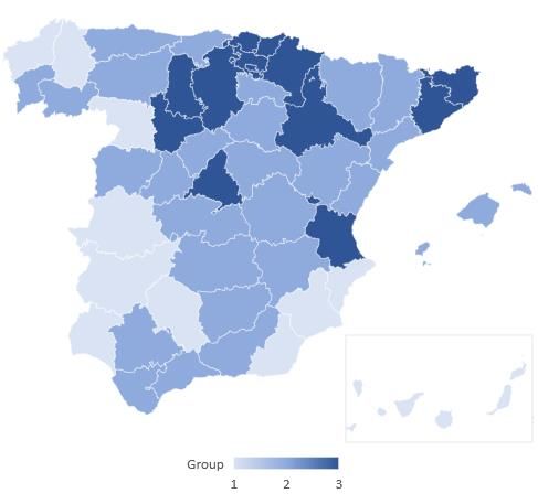
Annex 3: Spatial ECI distribution by group of provinces

Figure A.3: ECI by region and trade flow (1995)

 Panel A: Low-complexity regions Panel B: Mid-complexity regions

 Panel C: High-complexity regions Panel D: Total complexity of regions

Panels A–C: Each colour bar represents a region. Black lines represent minimum
and maximum complexity in each trade flow. The dotted line represents the
group’s median.

Panel D: Group 1 refers to low-complexity regions (first quartile), group 2 refers
to mid-complexity regions (second and third quartiles) and group 3 to the high-
complexity regions (fourth quartile).
Source: Own elaboration.

Annex 4. Econometric results.

Table A.4.1: GDP per capita growth (t+10) and (t+15) by province. Growth
 relative GDPpc. Cross-sections every t+10 and t+15 years. OLS estimator.

 1995-2005, 2005-2015 1995-2010

 M1 M2 M3 M4 M1 M2 M3 M4

Year FE YES YES YES YES YES YES YES YES

VARIABLES Regional GDPpc/World GDPpc (t+10) Regional GDPpc/World GDPpc (t+15)

Total ECI 0.537*** 0.530*** 0.524*** 0.414*** 0.396*** 0.456***
 (0.0768) (0.0792) (0.0773) (0.0847) (0.0857) (0.0875)
Physical cap. 0.173 0.146 0.149** 0.138 0.0512 0.268***
 (0.114) (0.139) (0.0688) (0.141) (0.174) (0.0760)
Human cap. -0.0424 0.181 0.0596 0.172 0.320** 0.266***
 (0.109) (0.132) (0.0679) (0.121) (0.150) (0.0522)

Observations 100 100 100 100 50 50 50 50
R-squared 0.505 0.244 0.484 0.504 0.544 0.284 0.526 0.514

Change in R-
 51.68% 4.16% 0.20% 47.79% 3.31% 5.51%
squared

Robust standard errors in
parentheses.
*** p

Table A.4.2: GDP per capita growth (t+10) and (t+15) by province.
 Absolute growth of GDPpc. Cross-sections every t+10 and t+15 years. OLS
 estimator.

 1995-2005, 2005-2015 1995-2010

 M1 M2 M3 M4 M1 M2 M3 M4

Year FE YES YES YES YES YES YES YES YES

VARIABLES GDP per capita (t+10) GDP per capita (t+15)

Total ECI 0.562*** 0.555*** 0.548*** 0.535*** 0.528*** 0.547***
 (0.0775) (0.0805) (0.0788) (0.103) (0.102) (0.100)
Physical cap. 0.190 0.162 0.165** 0.0479 -0.0648 0.0875
 (0.118) (0.144) (0.0711) (0.167) (0.213) (0.0812)
Human cap. -0.0445 0.189 0.0679 0.0527 0.245 0.0851
 (0.114) (0.137) (0.0700) (0.146) (0.186) (0.0618)

Observations 100 100 100 100 50 50 50 50
R-squared 0.427 0.124 0.400 0.426 0.439 0.080 0.438 0.437

Change in R-
 70.96% 6.32% 0.23% 81.78% 0.23% 0.46%
squared

Robust standard errors in parentheses
*** p

Table A.4.3: GDP per capita growth (t+5) by province. Growth relative
 GDPpc. Panel-data fixed effects estimations. OLS and within-groups’
 estimator.

 M5 M6 M7 M8
 Within- Within-
 OLS OLS Groups FE Groups FE
 TIME FE YES YES YES YES
 REGIONAL FE NO YES YES YES

 Regional GDPpc/World GDPpc t+5 t+15

 Total ECI 0.305*** 0.623*** 0.144** 0.116***
 (0.0241) (0.0717) (0.0625) (0.0425)
 Physical cap. 0.400*** 0.0836 -0.627*** -0.235***
 (0.0365) (0.0637) (0.0434) (0.0838)
 Human cap. 0.233*** 0.177*** 0.298*** -0.177***
 (0.0419) (0.0471) (0.0252) (0.0409)

 Observations 850 850 850 350
 R-squared 0.645 0.913 0.586 0.406
 Number of groups 50 50

 Robust standard errors in parentheses
 *** p

Table A.4.5: GDP per capita growth (t+5) and (t+15) by province. International, inter-regional and intra-regional EC
 indices. Growth relative GDPpc. OLS and within-groups’ estimator.

 M5 M5 M5 M6 M6 M6 M7 M7 M7 M8 M8 M8
 Within- Within- Within- Within- Within- Within-
 Groups Groups Groups Groups Groups Groups
 OLS OLS OLS OLS OLS OLS FE FE FE FE FE FE
 Inter- Intra- Inter- Intra- Inter- Intra- Inter- Intra-
ECI type International regional regional International regional regional International regional regional International regional regional
TIME FE YES YES YES YES YES YES YES YES YES YES YES YES
REGIONAL FE NO NO NO YES YES YES YES YES YES YES YES YES

VARIABLES Regional GDPpc/World GDPpc (t+5) Regional GDPpc/World GDPpc (t+15)

ECI 0.138*** 0.305*** 0.320*** 0.546*** 0.449*** 0.290*** 0.0630 0.0798* 0.0724* 0.172*** 0.0762** -0.0120
 (0.0232) (0.0260) (0.0252) (0.0825) (0.0614) (0.0428) (0.0777) (0.0475) (0.0389) (0.0538) (0.0308) (0.0263)
Physical cap. 0.414*** 0.406*** 0.378*** 0.126* 0.0607 0.00965 -0.634*** -0.634*** -0.630*** -0.270*** -0.217** -0.238***
 (0.0375) (0.0363) (0.0367) (0.0743) (0.0654) (0.0728) (0.0454) (0.0450) (0.0448) (0.0872) (0.0859) (0.0881)
Human cap. 0.354*** 0.230*** 0.284*** 0.223*** 0.200*** 0.224*** 0.295*** 0.299*** 0.297*** -0.165*** -0.186*** -0.184***
 (0.0439) (0.0408) (0.0366) (0.0534) (0.0510) (0.0513) (0.0259) (0.0261) (0.0249) (0.0408) (0.0416) (0.0423)

Observations 850 850 850 850 850 850 850 850 850 350 350 350
R-squared 0.599 0.645 0.664 0.894 0.902 0.892 0.580 0.583 0.585 0.417 0.401 0.388
Number of
groups 50 50 50 50 50 50

Robust standard errors in parentheses
*** p

GETTING IN TOUCH WITH THE EU
In person
All over the European Union there are hundreds of Europe Direct information centres. You can find the
address of the centre nearest you at: https://europa.eu/european-union/contact_en
On the phone or by email
Europe Direct is a service that answers your questions about the European Union. You can contact this
service:
- by freephone: 00 800 6 7 8 9 10 11 (certain operators may charge for these calls),
- at the following standard number: +32 22999696, or
- by electronic mail via: https://europa.eu/european-union/contact_en
FINDING INFORMATION ABOUT THE EU
Online
Information about the European Union in all the official languages of the EU is available on the Europa
website at: https://europa.eu/european-union/index_en
EU publications
You can download or order free and priced EU publications from EU Bookshop at:
https://publications.europa.eu/en/publications. Multiple copies of free publications may be obtained by
contacting Europe Direct or your local information centre (see https://europa.eu/european-
union/contact_en).