MicroVelocity: rethinking the Velocity of Money for digital currencies
←
→
Page content transcription
If your browser does not render page correctly, please read the page content below
MicroVelocity: rethinking the Velocity of Money
                                                        for digital currencies
arXiv:2201.13416v1 [econ.GN] 31 Jan 2022

                                            Carlo Campajola1,2 , Marco D’Errico∗3 , and Claudio J. Tessone1,2
                                                   1
                                                  University of Zurich, Blockchain & Distributed Ledger
                                              Technologies, Department of Informatics, Zürich, Switzerland
                                                     2
                                                       UZH Blockchain Center, Zürich, Switzerland
                                             3
                                               European Systemic Risk Board Secretariat, European Central
                                                                Bank, Frankfurt, Germany

                                                                              February 1, 2022

                                                                                    Abstract
                                                     We propose a novel framework to analyse the velocity of money in
                                                 terms of the contribution (MicroVelocity) of each individual agent, and
                                                 to uncover the distributional determinants of aggregate velocity. Leverag-
                                                 ing on complete publicly available transactions data stored in blockchains
                                                 from four cryptocurrencies, we empirically find that MicroVelocity i) is
                                                 very heterogeneously distributed and ii) strongly correlates with agents’
                                                 wealth. We further document the emergence of high-velocity interme-
                                                 diaries, thereby challenging the idea that these systems are fully decen-
                                                 tralised. Further, our framework and results provide policy insights for
                                                 the development and analysis of digital currencies.
                                               Keywords: Velocity of Money, Cryptocurrency, Blockchain, Heterogeneous agents
                                               JEL Classification: C81, D31, E41

                                           Introduction
                                           One of the earliest and most widespread concepts across societies is that of
                                           money. As humans we are inherently brought to organise ourselves into com-
                                           munities and exchange the goods and services we produce; this leads to the
                                           necessity to invent a medium of exchange that can be store of value - to be able
                                           to defer purchases to the future - and unit of account - to properly quantify the
                                           value of goods and services [1]. Any such artifact, which may take the form of
                                              ∗ The views expressed in this paper are those of the authors and do not necessarily reflect

                                           those of the ECB, the ESRB or its member institutions.

                                                                                         1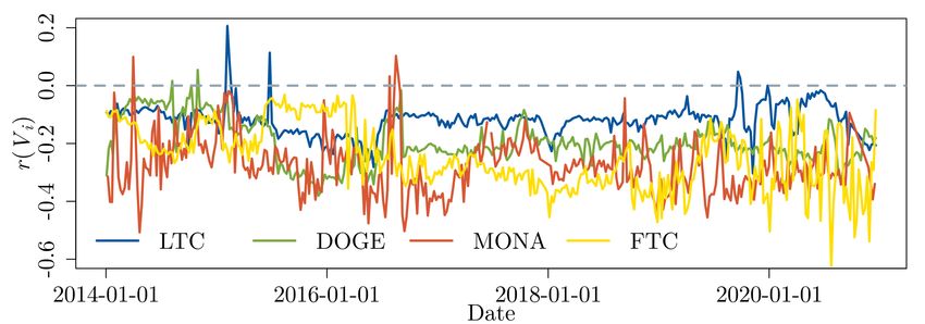
anything between a large stone in the middle of the village [2], cigarettes [3],
cash in the form of coins and banknotes or an encrypted sequence of bits [4], is
a form of money, as long as there is more than one person willing to accept it
as such.
     Over the years, economic theory has kept interrogating itself on how to
efficiently manage this peculiar asset: who is entitled to create it, what is its cost
and, most importantly, the role of money on societal and economic development.
These and other questions led to the development of monetary theory, which
interrogates on how the quantity of money in a system influences economic
activity and macroeconomic quantities.
     One of the main research areas in monetary theory is the quantity theory of
money, which revolves around Fisher’s equation of exchange [5]

                                     MV = PQ                                      (1)
    stating the proportionality between the monetary mass M and the level of
prices P through the economic output Q and V , the velocity of money. The
latter is defined as the average frequency with which a given unit of money is
used to purchase domestically-produced goods and services within a given time
period: this makes Fisher’s equation an accounting identity which holds true by
construction as both sides amount to the total money flow, which we will call
F . The velocity V is often seen as an indicator of money demand [6]: if money
demand is low - i.e. expected yield from alternative assets is high - economic
agents will convert their money into less liquid investments as soon as possible,
thus leading to increased velocity, whereas in situations of high demand for
money the velocity will decrease.
    Money velocity is not directly measurable since it would be impossible to
track every unit of currency circulating in the economy. Therefore, the equation
of exchange provides a way to estimate velocity at a given point in time. The
equation however holds true in aggregate, thus providing limited insights on the
distributional aspects, in particular for what concerns a more granular mea-
surement of velocity and how different economic agents (or groups of agents)
contribute to the aggregate. In fact, agents are heterogeneous, have different
spending habits, different levels of wealth, income and demand for money and
different roles in its movement in the economy; but since their different contribu-
tions to aggregate velocity are not measurable, policy analysis and interventions
cannot be targeted at a finer level.
    However, these limitations to the measurement of velocity might be not
so strict anymore: over the last few years the increasing diffusion of digital
payments - via electronic cards, e-banking or smartphone apps, to name some
alternatives - has led to a surge in transactions data availability, meaning that it
is now within reach to actually measure the velocity of money from micro-level
data, at least for digital forms of money. A big role in this transition towards
digital cash will be played by central banks, who are now devoting significant
resources towards the development of Central Bank Digital Currencies (CBDCs)
[7, 8, 9] to provide citizens with access to central bank money in digital form.

                                          2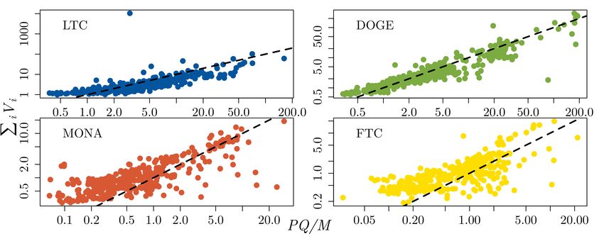
A strong push towards digital payments has been prompted by the rise
over recent years of cryptocurrencies and blockchain-based tokens. These have
emerged as a family of unconventional financial assets and some of them, with
Bitcoin being the first and most prominent example, claimed they could be
the future of money and would take over the role of fiat currencies. While
this has not happened, and outside of crypto-maximalist communities it is now
commonplace not to consider Bitcoin and its many offsprings as currencies,
the publicly available records of blockchains constitute a unique opportunity
to explore the space of microeconomically grounded metrics for macroeconomic
quantities like the velocity of money.
    In particular in this paper we focus on exploiting the accounting protocol
adopted by several cryptocurrencies, the Unspent Transaction Output (UTXO)
protocol, to actually track specific units of currency as they move from one agent
to the other. This protocol imposes that whenever funds have to be spent they
are included as inputs of a transaction, and they have explicit reference to the
unspent output of a previously validated transaction. This provides verification
that the issuer of the new transaction has the right to spend those funds, as
the output can only be accessed by means of a cryptographic private key owned
by the receiver. A by-product of this mechanism is that every input to a new
transaction is explicitly linked to the output of a previous one, and thus the
time that those units of money stayed idle is known.
    As we explain in the following, this level of detail allows to factor the total
velocity V into agent-specific contributions, Vi , which we call MicroVelocity
and depend on agents’ behavioral usage of their wealth. This description, based
on the seminal work of [10], opens to several questions: how is MicroVelocity
distributed cross-sectionally? How does it evolve over time? How does an
agent’s MicroVelocity correlate with their wealth? How does it correlate with
the MicroVelocity of their partners in transactions?
    In the context of cryptocurrencies, the velocity of money has been used to
propose valuation models [11, 12], by an argument stating that if the economy
adopting cryptocurrency as its medium of exchange grows, so does the velocity
due to the available supply being limited by protocol, thus an increase in ve-
locity should also warrant an increase in pricing. Several estimators have been
proposed for the velocity of cryptocurrencies, like Coin Days Destroyed [13] or
Average Dormancy [14]. In particular Pernice et al. [15] propose an accurate
method to estimate velocity on aggregate, which takes advantage of the UTXO
protocol in similar ways to our definition of MicroVelocity.
    We argue that MicroVelocity allows more detailed considerations on the state
of the economy using cryptocurrencies. Specifically, statistical properties of its
distribution across agents provide insight into the global level of specialization
and on centralization in the flow of money: if the distribution is highly het-
erogeneous, agents with high MicroVelocity are likely to be intermediaries and
those with low Vi their clients, thus going against the common narrative that
cryptocurrencies are “decentralized economies". Paths towards the centraliza-
tion of these systems are currently attracting growing attention, with Aramonte
et al. [16] explicitly talking of “decentralization illusion".

                                        3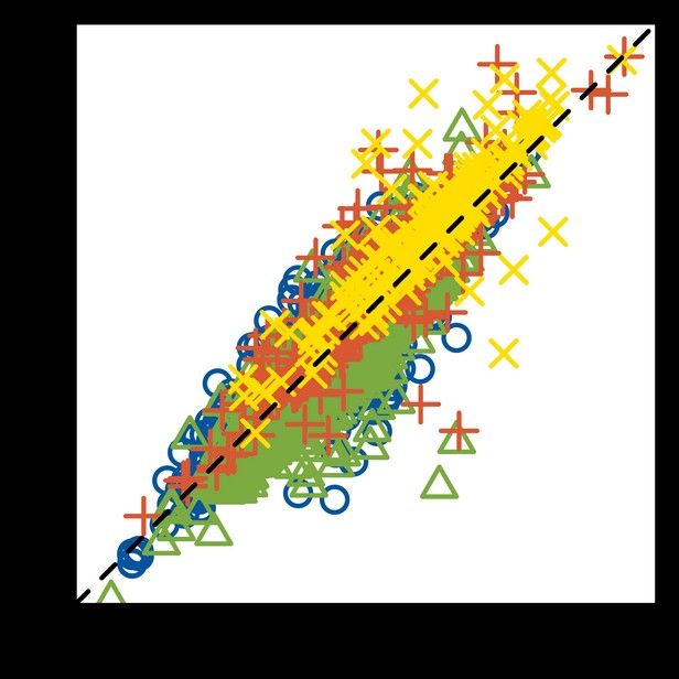
Regardless, our framework is not necessarily limited to the context of blockchain-
based tokens. The formulation of MicroVelocity general in nature and can be
adapted to find application to any payment system that keeps a digital record
of transactions, such as bank transfers, credit cards payments or, in the future,
CBDCs. Such an instrument will then be a useful addition to economists’ tool-
boxes when investigating effects of policy, and possibly even opening new policy
channels that account for the heterogeneity of economic agents in their usage of
money [17, 18].

MicroVelocity. We build on Wang and coauthors’ theoretical framework [10],
which shows that the macroeconomic velocity can be derived from a microeco-
nomic description: here we review and expand their argument, introducing our
definition of MicroVelocity.
    Consider the time between two transactions involving the same unit of cur-
rency, the holding time τ , and assume that τ is a random variable with proba-
bility distribution p(τ ). A condition p(0) = 0 has to be enforced since a holding
time of 0 is meaningless for the description. It follows that, calling M the total
number of coins in circulation, M p(τ )dτ is the number of coins with a holding
time in the interval [τ, τ + dτ ).
    Assuming stationarity of p(τ ), the money flow F (τ ) generated by coins with
holding time τ is
                                          1
                                F (τ ) = M p(τ )dτ                           (2)
                                          τ
    as 1/τ is the frequency with which each coin moves. Since the total economic
flow F is the integral of this quantity over all holding times, we find
                                              Z ∞
                                                   1
                        F = MV = PQ = M              p(τ )dτ                 (3)
                                               0   τ
   and it thus follows that the velocity reads
                                   Z +∞
                                          1
                              V =           p(τ )dτ                            (4)
                                    0     τ
    It has to be noticed that units of currency are not distinguishable and there
is no reason to think that a particular coin has an inherently different holding
time than any other one. Indeed the authors of [10] justify the existence of
the holding times distribution by arguing that holding times depend on money
ownership, i.e. the spending habits of different economic agents produce the
heterogeneity in τ . While coins are indistinguishable, economic agents are not
and each has their own spending, saving and speculative attitude.
    In the original paper the authors only consider the aggregate effect of this
heterogeneity, defining p(τ ) but neglecting to consider the individual effects
of agents, as a simulation study accounting for it would have introduced too
many arbitrary parameters in the description. Our goal is thus to overcome this

                                        4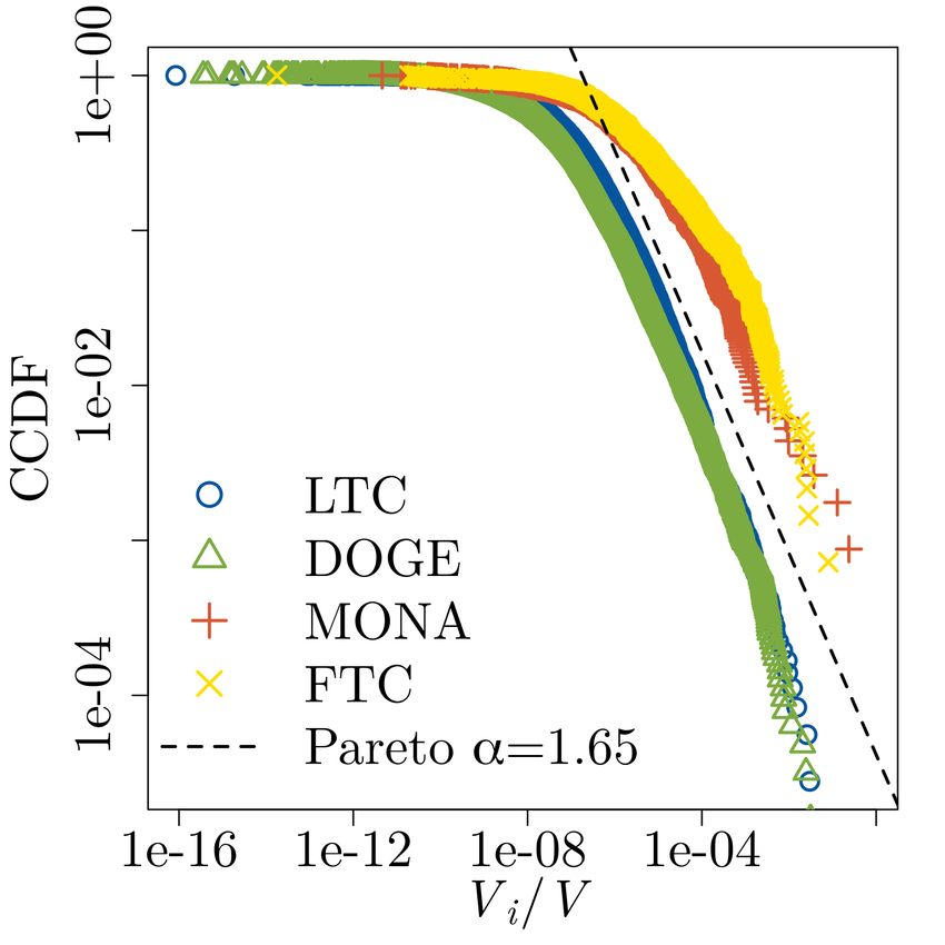
limitation, as having access to agent-level data allows for a more fine-grained
representation.
    Let us then define pi (τ ) as the probability distribution of holding times of
agent i, with i ∈ {1, 2, . . . N }. This means that the total flow of Eq. 3 is factored
in a sum of individual contributions, and then Eq. 4 transforms into
                              N            N    Z        ∞
                              X            X Mi              1
                        V =         Vi =                       pi (τ )dτ           (5)
                              i=1          i=1
                                                 M   0       τ
    where Mi is the amount of money held by agent i, meaning that the total
velocity is a wealth-weighted average of individual contributions, the MicroVe-
locity Vi . This equation makes it clear that, in a population with homogeneous
spending preferences such that pi (τ ) ≈ p(τ ) ∀i, contributions to money ve-
locity are fully determined by wealth. However real-world economies involve
heterogeneous participants, both on the macro-scale (households, companies,
business sectors) and on the micro-scale (preferences, consumption functions):
our framework fully accounts for these factors, returning a detailed picture of
the impact they have on the velocity.

Blockchains and the UTXO protocol. To estimate MicroVelocity from
real-world data one needs fine-grained transaction records, so that the holding
times τ can be measured and its statistical properties estimated. The advent
of blockchains and cryptocurrencies offers a unique occasion to study economic
activity on a publicly available transaction ledger. A blockchain is a distributed
ledger used to store information upon which a large community agrees without
having a central authority that coordinates the consensus. Avoiding going into
the details of how the consensus protocol works, what matters for this paper is
the accounting standard that is used to store the data on the blockchain. There
are several alternatives that are currently being used, but the most popular so
far - and first to be implemented in Bitcoin - is the Unspent Transaction Output
(UTXO).
    In this protocol, schematised in Fig. 1, information is stored on the blockchain
in form of transactions, transferring usage rights of some quantity of digital as-
set from one cryptographic address to another. These addresses consist of two
parts: a public key, visible to everybody and used for verification, and a private
key, which is information only available to the address owner. When an agent
wants to transfer some assets to another agent, they need to point to a previ-
ously generated transaction output that has not been spent yet and, using their
private key, demonstrate that they own the address that output was destined
to. This shows they own the usage rights on the assets in that output, and
they are able to transfer them by pointing to an address belonging to the new
transaction receiver.
    Since all this information is stored on the blockchain, this means that the
time occurring between the generation of the UTXO and its spending transac-
tion is easily available, thus allowing to measure τ for all coins without further
assumptions. These can then be used to estimate pi (τ ) depending on ownership,

                                                 5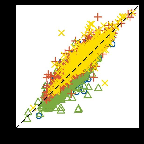
transactions         generation transaction
                                                  #6                         25/03/14 01:36        #7                25/03/14 02:24   #8                25/03/14 03:12
 # block height            block time               61                                             71                                 81
  A                                                coinbase       25       O61 [1]        25       coinbase   25   O71 [1]     25                25               25
                                                                                                                                      coinbase        O81 [1]
  coinbase       25     OA [1]          25
                                                    62                                             72                                 82
  B                                                O42 [1]        15       O62 [1]        8        O62 [1]    8    O72 [1]     7                                  10
                                                                                                                                      O63 [1]    11   O82[1]
                                                                                                                                                      O11 [1]     15
 OZ [2]          10     OB [1]          10                                 O62 [2]        7                        O72 [2]     1                      O82 [2]     1
                                                    63                                             73
  C                                                                                                                                   83
                 2                      3          O32 [2]        11       O63 [1]        11       O62 [2]    7    O73 [1]     5
 OX [1]                 OC [1]                                                                                                        O73 [2]    4    O83 [1]     3
                 4                      1                                                          O54 [1]    2    O73 [2]     4
 OY [3]                 OC [2]                      64                                                                                O64 [1]    4    O83 [2]     3
                        OC [3]          2                                                                                                             O83 [3]     2
                                                   O23 [1]        4        O64 [1]        4
        inputs               outputs
 spent output [position] and value,            transaction output [position] and value,
 cryptographically signed                      with public signature of the recipient

Figure 1: Schematic representation of a UTXO blockchain. Each block contains
transactions, in turn consisting of a set of inputs and outputs. Total input and output
values must be matching. An output grants usage rights of some amount of tokens to
an address, identified by its public key. Inputs are references to unspent outputs from
previous blocks, cryptographically signed by matching the public and private keys. A
coinbase transaction generates new tokens as reward to the miner of the block.

thus providing all the necessary information to calculate the MicroVelocity of
Eq. 5.

Measuring MicroVelocity on blockchains. Events are recorded on the
blockchain once every few minutes, when a new block is added. The consequence
is that time is effectively discretised, and τ can be expressed in terms of number
of blocks between transactions, τ ∈ N \ {0}. Following the logic above, let us
define Pi (τ ) to be the probability mass function of the discrete holding times
for user i’s coins. Then Mi Pi (τ ) coins by user i have holding time τ , resulting
at stationarity in a contribution to user i’s flow of
                                        1
                                          Mi Pi (τ )                     Fi (τ ) =
                                       τ
   It then follows that the total velocity, given in continuous time by Eq. 5,
turns into the following formula in block time
                                                                                 N X ∞
                                                                                X        Mi 1
                                                                   V =                        Pi (τ )                                                             (6)
                                                                                i=1 τ =1
                                                                                         M τ
   Isolating the i-th component of this sum we are then able to define user i’s
contribution to the macroeconomic velocity of money, i.e. the MicroVelocity,
which is
                                                                                       ∞
                                                                                      X    Mi 1
                                                                        Vi =                    Pi (τ )                                                           (7)
                                                                                      τ =1
                                                                                           M τ

    The question is then how to measure Pi (τ ) to be able to compute these
quantities. For the specific case of UTXO-based cryptocurrencies, a very simple
estimator can be adopted: the accounting protocol itself produces the holding
time τ of each unit of currency as a by-product, hence the empirical probability
of these holding times conditional on the agent can be estimated. For example,

                                                                                               6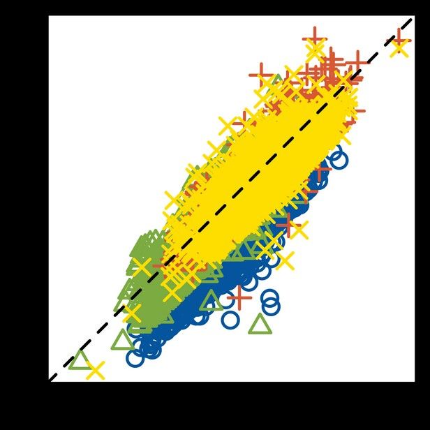
in Fig. 1, the inputs of transaction 83 have the same value (4 tokens) but
different holding time of two blocks (O64[1]) and of one block (O73[2]). This
means, according to Eq. 7, that tokens in O64[1] generate half as much velocity
as the ones in O73[2].
    There are two further cautions that need to be mentioned. The first is that
in principle there is no guarantee that a transaction recorded on the blockchain
is actually a transfer of value from an agent to another: addresses do not have a
one-to-one correspondence with agents’ wallets, and in fact a wallet can contain
an arbitrary number of addresses. Moreover, by protocol, inputs of transactions
have to be spent in full each time: the total value of inputs has to match the
total value of outputs, and the value of inputs is constrained by the UTXO they
point to. The way in which this is solved is by generating an extra output, called
change output, which points the excess input to an address which is actually
owned by the sender. These transactions do not actually move funds between
individuals, thus they should be excluded from the calculation of MicroVelocity.
    To solve this issue, when we find an output that is likely to belong to
the transaction sender, we do not count it on the MicroVelocity and add the
weighted average holding time of the inputs of that transaction to its hold-
ing time. There are several ways to identify self-transactions through heuristic
methods which take advantage of typical patterns used by cryptocurrency wal-
let clients. We provide further details about this in the Materials and Methods
section.
    The second caution that is needed is that, when calculating MicroVelocity,
the measurable holding times are right-censored, or in other words one would
need future information to know the holding time of current UTXOs. While
there is no straightforward solution to this, it is in principle possible to devise
more refined statistical methods to infer Pi (τ ) so that one can reduce this issue,
while also controlling for the impact of non-stationarity in the estimation, which
we have neglected in this work. We choose not to tackle this problem, as it would
require some arbitrary assumptions, and defer the exploration of solutions to
future research.

Materials and Methods
Data processing. We directly collect data from the Litecoin, Dogecoin, Mona-
coin and Feathercoin blockchains by synchronizing full nodes in archive mode.
The complete history has then been preprocessed using the Blocksci Python
library [19], which turns raw data files into an efficiently searchable database
structure.
    There are many heuristic methods that have been proposed to assign ad-
dresses to unique wallets. Here we combine three heuristics, the MultiInput
(MI), the Change Address (CA) and the Peeling Chains (PC):
   • MI takes advantage of the fact that multiple addresses appearing as inputs
     of the same transaction have a high likelihood of belonging to the same
     agent, as they had to be signed with all the private keys together. For

                                         7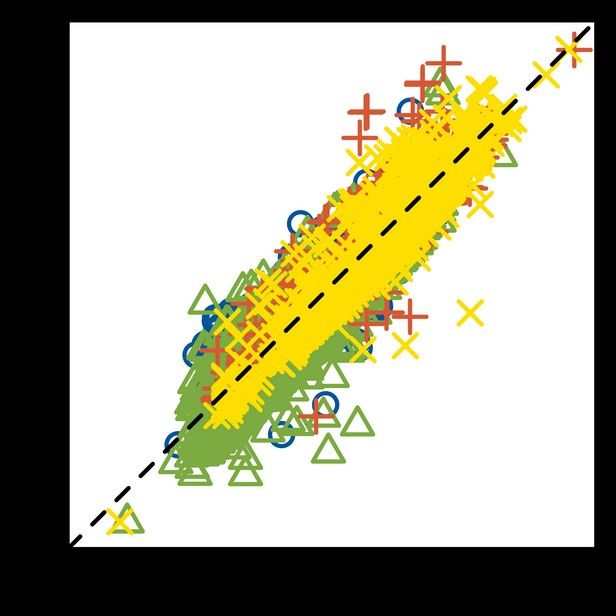
example in Fig. 1, O64[1] and O73[2] are assigned to the same wallet
      since they appear together as inputs of transaction 83;
   • CA follows from the argument that, when there is more than one input
     and more than one output in a transaction, it is likely that the smallest
     output is a change address, provided it is smaller than the smallest input
     (otherwise such input would have not been necessary) and that it is a new
     address; if one such output is identified, it is considered to belong to the
     same agent as the input addresses. In Fig. 1, output O83[3] is likely a
     change address and is associated with O64[1] and O73[2];
   • Finally, PC identifies transaction patterns called peeling chains: sequences
     of transactions with a single input and two outputs, that arise when an
     agent needs to spend a large value UTXO (like a coinbase transaction),
     generating chains of transactions where the UTXO is slowly consumed. In
     order to identify a peeling chain, at least two subsequent transactions have
     to match this pattern. If that is the case, the outputs that connect the
     chain are assigned to the same wallet as the inputs. In Fig. 1, transactions
     62 and 72 constitute a peeling chain, hence addresses O42[1], O62[1] and
     O72[1] are linked with one wallet.
    When using heuristics to cluster together output and input addresses, there
is a significant risk of merging multiple wallets together. For this reason we
adopt some logical selection rules to limit the impact of this issue. In particular
we apply the following conditions:
   • if different heuristics disagree on the change address, no change address is
     selected;
   • if all heuristics agree on the change address or select none, that address is
     considered the change;
   • if an input address appears also in the output, it is necessarily the change
     and all heuristics are neglected.

Estimation of MicroVelocity. The estimation of MicroVelocity follows from
the sum of Eq. 7. At a given time t, an agent owns Mi (t) coins, each with some
holding time τ that is estimated as the age of the UTXO they are included in
when they are spent. Then the time t probability mass function of holding times
of agent i, Pit (τ ), is measured as the empirical probability

                                              wi (τ )
                                 Pit (τ ) =
                                              Mi (t)
where     wi (τ ) is the total value of UTXOs with holding time τ , ensuring that
            ) = Mi (t). Plugging this into Eq. 5 gives the empirical value of agent
P
   τ w i (τ
i’s MicroVelocity at time t
                                            X 1 wi (τ )
                                   Vi (t) =
                                            τ
                                              τ M (t)

                                         8
Figure 2: Comparison of total MicroVelocity and the ratio of total flow to monetary
mass P Q/M , with weekly aggregation. All quantities are annualised.
where M (t) is the total amount of money in the system at the time. Notice
that this value is known by construction, since the supply of cryptocurrencies
is deterministic. We neglect additional considerations on the definition of circu-
lating supply, as they would require arbitrary assumptions and we believe they
would have a marginal impact on our results. Indeed, since the holding time
τ appears at the denominator of Eq. 7, coins with a longer holding time that
may be classified in less liquid monetary aggregates already contribute less to
the velocity.
Results
The distribution of MicroVelocity. We begin our analysis by checking if
the total MicroVelocity we measure correctly matches the velocity calculated
following Fisher’s Eq. 1. In Figure 2 we compare the sum of MicroVelocities
, averaged weekly, with the average volume of transactions P Q divided
P
i Vi
by the total money supply M on that week. Both quantities are annualised to
facilitate comparison. It appears clear that Eq. 6 holds true, with the total
MicroVelocity even producing a slightly less volatile estimate of V . This is not
surprising, since MicroVelocity accounts for components of V at all timescales
whereas P Q/M only considers transactions happening on a specific time window
(in this case a week), thus being more prone to temporary fluctuations.
However, as discussed above, the advantage of having this microeconomic
picture is that we are able to investigate the distributional aspects of the velocity
of money. We then proceed to take weekly cross-sectional snapshots of the
agents’ Vi s, which we then utilize to extract a number of statistics and test
hypotheses. First, we remove values of Vi (t) = 0 from our analysis. These may
occur for multiple reasons: the agent may have not entered the market yet or
has quit, thus they will have 0 wealth and velocity, but it may also be that
they own coins which they never spend. The latter can itself be caused by a
9LTC DOGE MONA FTC
Mean 1.69 1.65 1.56 1.62
Min. 1.44 1.52 1.28 1.27
Q1 1.64 1.61 1.52 1.52
α
Median 1.70 1.65 1.55 1.59
Q3 1.74 1.68 1.61 1.69
Max. 1.92 1.80 2.29 2.20
Mean 0.03 0.03 0.08 0.11
DP ar
p > 0.2 92.96% 100.00% 99.92% 94.07%
Mean 0.83 0.86 0.83 0.78
DExp
p > 0.2 0% 0% 0% 0%
Figure 3 & Table 1: (left) Snapshot of complementary cumulative distribution func-
tion (CCDF) of relative MicroVelocity Vi /V on April 4th, 2016 for the four cryptocur-
rencies. A Pareto distribution with tail exponent α = 1.65 is reported as comparison.
(right) Pareto fit and Kolmogorov-Smirnov test. Summary statistics - mean, quartiles,
minimum and maximum - for the estimated α parameter of the Pareto distribution
and for the K-S tests. The “p > 0.2" lines report the percentage of two-tailed K-S
tests that don’t reject the Pareto and Exponential nulls at the 20% confidence level.
Critical values obtained by bootstrap.
behavioral choice of holding the coins indefinitely - the so-called “HODLers" -,
by the right-censoring of data we previously discussed or by technical problems
such as lost passwords or hacks: this uncertainty leads us to exclude also agents
with non-zero wealth that have zero MicroVelocity.
We then proceed to analyze the cross-sectional distribution by means of the
Kolmogorov-Smirnov distance D from a known distribution. This is defined as
D = sup|P̂ (Vi ) − P (Vi )|
where P̂ (Vi ) is the empirical distribution of MicroVelocities and P (Vi ) is an
arbitrary probability distribution. This distance is the test statistic for the two-
tailed Kolmogorov-Smirnov test, which tests the null hypothesis that P̂ (Vi ) ≡
P (Vi ). Since Vi ≥ 0 by definition, we choose to take as comparisons the expo-
nential and Pareto distributions, to gain insight on whether the data is closer
to a thin- or to a fat-tailed distribution. We fit the parameters of these dis-
tributions by Maximum Likelihood methods and calculate the distances DP ar
and DExp , obtaining the results summarized in Table 3. While the thin-tailed
exponential null hypothesis is always rejected by the Kolmogorov-Smirnov test,
it is clear that a fat-tailed Pareto distribution with tail exponent α ≈ 1.6 is
a much better descriptor for the distribution generating the data. Notice that
we choose a very high significance threshold of 0.2, since we want to check the
robustness of the null hypothesis rather than identifying an alternative. Despite
this, the test almost never rejects the Pareto null, consolidating the observation
that the total velocity of money is very unevenly distributed across agents, with
a small minority dominating the sum of Eq. 7.
Perhaps the most striking evidence of this comes from the stacked charts
of Fig. 4. In each panel’s bottom chart, each colored area corresponds to the
10Figure 4: Area charts of MicroVelocity and identity of top 5 individual contributors
for the four cryptocurrencies, averaged weekly. In each panel the top chart shows
the frequency (vertical axis) with which the 5 most represented agents (horizontal
axis) figure in the top 5 contributors, with stacked bars colored to show their ranking
according to the legend. The bottom charts show the share of V contributed by the
top 5 agents as a function of time. We see that one agent is always in the top 5 and
that in all cases the vast majority of the total velocity is concentrated in the hands of
a few agents.
fraction of total velocity that is produced by the 5 largest contributors, com-
pared with the total contributions by all others, tracked over time with weekly
aggregation. In all the analyzed cryptocurrencies the vast majority of the total
velocity is generated by less than 5 agents: most likely these - whose actual
identity is unknown to us - are companies that act as intermediaries, such as
exchange markets, custodians or layer 2 payment services like the Lightning
Network [20]. Despite the real-world identity of these agents being unknown,
we can still track them by their ID from the address clustering algorithm, which
means we are able to count how frequently each agent features as a top con-
tributor. The top charts of Fig. 4 show exactly this, counting the percentage
of weeks a given agent is among the top 5 and showing their ranking with the
colored bar. It appears that only one agent is always in the top 5, most of
the times as top contributor, whereas others show significantly less persistence.
This is most likely due to our choice of heuristics for address clustering, which
possibly clusters together multiple exchanges.
MicroVelocity and wealth. While we have no information about the real-
world identities of agents, we can still characterize them by their activity on
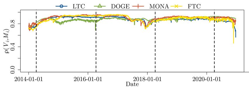
11Figure 5: Spearman’s rank correlation between the MicroVelocity Vi and the wealth
Mi of the agent. Insets: scatterplots of Vi /V vs Mi /M in log-log scales at marked
dates, with dashed line on the diagonal Vi /V = Mi /M .
the blockchain and see how their features correlate with their MicroVelocity.
In particular we focus on the relation arising between MicroVelocity and agent
wealth Mi . As mentioned when we introduced Eq. 5, in an economy where the
“consumption functions" incorporated Pi (τ ) are homogeneous, Mi would be the
only factor to generate diversity in MicroVelocity. The systems we analyze have
high wealth concentration, which is a tendency that is common to cryptocur-
rencies [21, 22, 23, 24]. This is likely due to large pseudo-banking companies
that arise naturally in the environment, acting as exchange markets for fiat
currencies or as vaults where crypto users securely store their tokens [25]. In
Fig. 5 we show the Spearman’s rank correlation coefficient ρ between Vi and
Mi over time. We choose Spearman’s coefficient to overcome the limitation of
Pearson’s correlations for highly heterogeneous data (as discussed in the previ-
ous section), where outliers would taint the estimation of the correlation. Fig.
5 shows that the correlation is positive and consistently above 0.6. While it
is clear that Mi is a strong determinant of Vi , as expected from Eq. 5, there
is still a significant variance around the linear trend, as we show in the inset
scatterplots, and also variation over time. This residual variance is then entirely
due to the heterogeneity in Pi (τ ), which does not seem to be itself dependent on
wealth. One interesting phenomenon seems to appear during late 2017, with ρ
decreasing throughout the period of build-up of the crypto bubble that peaked
in December 2017 [26].
MicroVelocity and the structure of the economy. We conclude our anal-
ysis by considering the role of MicroVelocity in the structure of transaction pat-
terns, introducing transaction networks. A network is an ordered pair of sets
G = (V, E), called the nodes V and edges (or links) E, where the elements of
E ∈ V × V represent connections between elements of V. Identifying agents as
nodes and transactions as directed connections from the transaction sender to
the receiver, as done for instance in [27], it is possible to obtain a topological
description of the economy, highlighting with whom agents exchange tokens and
12Figure 6: Rank assortativity of MicroVelocity on weekly transaction networks.
how central they are in the flow of value in the economy. We construct trans-
action networks on weekly aggregation, which is the minimum timescale that
allows to mitigate the effect of day-of-the-week seasonalities that are common
in economic and financial data (e.g. weekend effects, higher volumes on Mon-
days/Fridays, etc.). Operationally this means that a connection from agent i to
agent j is present if at least one transaction occurred between them in a given
week. We then proceed to take the values of Vi at the end of each week and
assign them to each node as attributes, which then allows us to consider the
assortativity coefficient of these networks with respect to MicroVelocity.
The assortativity coefficient, defined by [28], is the Pearson correlation co-
efficient of a given node-specific quantity across linked pairs in a network. It
has been introduced to measure how nodes select their neighbors with respect
to specific characteristics, most prominently the degree, and it is defined as
P
(i,j)∈E (x(i) − hxi)(x(j) − hxi)
r= P 2
i∈V (x(i) − hxi)
where x(i) is the node-specific property of interest and h·i indicates the arith-
metic mean operator. A positive value of this coefficient indicates homophily,
i.e. links mainly connect similar nodes in terms of the selected property, whereas
a negative value indicates heterophily, i.e. connections mostly appear between
nodes with very different values of x.
In our case we decide to use the rank in MicroVelocity as the nodes attribute
x, thus computing a Spearman’s correlation instead of Pearson’s, again to ac-
count for the fat-tailed nature of the distribution of Vi s. We report our finding
in Fig. 6, where we plot this rank assortativity coefficient for MicroVelocity on
weekly networks as a function of time. The resulting measure is mostly nega-
tive, thus suggesting that highly-ranked nodes mostly trade with lowly-ranked
ones and vice-versa.
13Discussion
In this article we investigated the microeconomic foundations of the macroe-
conomic velocity of money, building upon theoretical work [10] and realizing
the first empirical measurement of the velocity of money from micro-level data.
We leveraged on the technological breakthrough provided by digital currencies
and by cryptocurrencies in particular, which offer unprecedented detail about
the movement of money in a closed economy where all coins can be followed in
every transaction they take part in. We have thus been able to introduce the
individual contribution to velocity by single agents, which we have called Mi-
croVelocity, as a function of the agent-conditional distribution of holding times
of money.
We argue that insights about the distribution and characterization of Mi-
croVelocity are valuable to researchers, policymakers and to the public to gain
a deeper understanding of the structure of the economy: in the particular case
at hand, we provide evidence that cryptocurrency economies’ claim of being
“decentralized" is largely unjustified, as shown by the extremely skewed distri-
butions of wealth and MicroVelocity we measure. This “decentalization illusion"
is unmasked by the highly heterogeneous MicroVelocity distribution, indicating
that few entities are intermediaries to most of the transactions, since large values
of MicroVelocity are easily due to high turnover in assets.
The fact that we find an extremely positive correlation between MicroVeloc-
ity and wealth, as well as negative assortativity of Vi in transaction networks, is
also corroborating evidence that these economies have seen the rise of pseudo-
banking services which centralize the supply of money and act as custodians
and intermediation services, often without any scrutiny by regulators due to
the lack of appropriate legislation.
We envision multiple directions that could be taken following this work,
tackling some limitations of our study as well as expanding its applicability
beyond the relatively narrow realm of UTXO-based cryptocurrencies.
The specific implementation we proposed here takes advantage of the fact
that holding times are relatively easy to compute thanks to the age of UTXOs,
but this can be easily overcome in the case where this information is not available
by considering, for instance, a Last-In-First-Out (LIFO) or First-In-First-Out
(FIFO) spending rule, as done for instance in [29]. We argue that a LIFO rule
is possibly the most economically significant for a medium of exchange, as it
would automatically exclude less liquid portions of the money supply from the
calculation, but we leave this extension for future research.
Our approach using empirical probabilities to estimate Pi (τ ) has a limita-
tion in the fact that holding times data is right-censored, and this becomes a
bigger issue the closer one is to present times. Moreover using empirical prob-
abilities does not fully respect the assumptions on stationarity; nonetheless the
convergence between the micro and macro quantities shown in Fig. 2 leads us
to think that they still are a good first approximation. We are confident that
these issues could be reduced by performing some additional assumptions on
the form of the holding times distribution, possibly giving it a parametric form
14justified by theory (e.g. the Gamma family proposed in [10]). This would mit-
igate the limitations and possibly allow to produce forecasts as well as predict
the outcome of policy interventions.
References
[1] S Mishkin Frederic. The economics of money, banking and financial mar-
kets. Mishkin Frederic–Addison Wesley Longman, 2004.
[2] Scott M Fitzpatrick and Stephen McKeon. Banking on stone money: an-
cient antecedents to bitcoin. Economic Anthropology, 7(1):7–21, 2020.
[3] Kenneth Burdett, Alberto Trejos, and Randall Wright. Cigarette money.
Journal of Economic Theory, 99(1-2):117–142, 2001.
[4] Satoshi Nakamoto. A peer-to-peer electronic cash system. Bitcoin.–URL:
https://bitcoin.org/bitcoin.pdf, 4, 2008.
[5] Irving Fisher. The purchasing power of money: its’ determination and
relation to credit interest and crises. Macmillan, New York, 1911.
[6] Milton Friedman. The demand for money: some theoretical and empirical
results. Journal of Political economy, 67(4):327–351, 1959.
[7] Walter Engert and Ben Siu-Cheong Fung. Central bank digital currency:
Motivations and implications. Technical report, Bank of Canada Staff Dis-
cussion Paper, 2017.
[8] Group of central banks. Central bank digital currencies: foundational
principles and core features. Technical report, Bank of Canada, Eu-
ropean Central Bank, Bank of Japan, Sveriges Riksbank, Swiss Na-
tional Bank, Bank of England, Board of Governors of the Federal Re-
serve System and Bank for International Settlements, 2020. available at
https://www.bis.org/publ/othp33.htm.
[9] European Central Bank. Report on a digital euro. ECB Report Series,
2020.
[10] Yougui Wang, Ning Ding, and Li Zhang. The circulation of money and hold-
ing time distribution. Physica A: Statistical Mechanics and its Applications,
324(3-4):665–677, 2003.
[11] Susan Athey, Ivo Parashkevov, Vishnu Sarukkai, and Jing Xia. Bitcoin
pricing, adoption, and usage: Theory and evidence. Stanford University
Graduate School of Business Research Paper, 2016.
[12] Wilko Bolt and Maarten RC Van Oordt. On the value of virtual currencies.
Journal of Money, Credit and Banking, 52(4):835–862, 2020.
15[13] Pavel Ciaian, Miroslava Rajcaniova, and d’Artis Kancs. The digital agenda
of virtual currencies: Can bitcoin become a global currency? Information
Systems and e-Business Management, 14(4):883–919, 2016.
[14] Reginald D Smith. Bitcoin average dormancy: A measure of turnover and
trading activity. Ledger, 3, 2018.
[15] Ingolf Gunnar Anton Pernice, Georg Gentzen, and Hermann Elendner.
Cryptocurrencies and the velocity of money. In Cryptoeconomic Systems
Conference, 2020.
[16] Sirio Aramonte, Wenqian Huang, and Andreas Schrimpf. Defi risks and
the decentralisation illusion. BIS Quarterly Review, 2021.
[17] Isabel Schnabel. Unequal scars - distributional consequences of the pan-
demic. Speech at Deutscher Juristentag 2020, 2020.
[18] H Ahnert, IK Kavonius, J Honkkila, and P Sola. Understanding household
wealth: linking macro and micro data to produce distributional financial
accounts. ECB Statistics Paper Series, 37, 2020.
[19] Harry Kalodner, Malte Möser, Kevin Lee, Steven Goldfeder, Martin Plat-
tner, Alishah Chator, and Arvind Narayanan. Blocksci: Design and ap-
plications of a blockchain analysis platform. In 29th {USENIX} Security
Symposium ({USENIX} Security 20), pages 2721–2738, 2020.
[20] Jian-Hong Lin, Kevin Primicerio, Tiziano Squartini, Christian Decker, and
Claudio J Tessone. Lightning network: a second path towards centralisation
of the Bitcoin economy. New Journal of Physics, 22(8):83022, aug 2020.
[21] Dániel Kondor, Márton Pósfai, István Csabai, and Gábor Vattay. Do the
rich get richer? an empirical analysis of the bitcoin transaction network.
PLOS ONE, 9(2):e86197, 2014.
[22] Garrick Hileman and Michel Rauchs. Global cryptocurrency benchmarking
study. Cambridge Centre for Alternative Finance, 33:33–113, 2017.
[23] Nicolò Vallarano, Claudio J. Tessone, and Tiziano Squartini. Bitcoin trans-
action networks: An overview of recent results. Frontiers in Physics, 8:286,
2020.
[24] Francesco Maria De Collibus, Alberto Partida, Matija Piškorec, and Clau-
dio J. Tessone. Heterogeneous preferential attachment in key ethereum-
based cryptoassets. Frontiers in Physics, 9, 2021.
[25] Ashish Rajendra Sai, Jim Buckley, Brian Fitzgerald, and Andrew Le Gear.
Taxonomy of centralization in public blockchain systems: A systematic
literature review. Information Processing & Management, 58(4):102584,
2021.
16[26] Nikolaos Kyriazis, Stephanos Papadamou, and Shaen Corbet. A system-
atic review of the bubble dynamics of cryptocurrency prices. Research in
International Business and Finance, 54:101254, 2020.
[27] Alexandre Bovet, Carlo Campajola, Francesco Mottes, Valerio Restocchi,
Nicolo Vallarano, Tiziano Squartini, and Claudio J Tessone. The evolving
liaisons between the transaction networks of bitcoin and its price dynamics.
arXiv preprint arXiv:1907.03577, 2019.
[28] Mark E.J. Newman. Assortative mixing in networks. Physical Review
Letters, 89(20):208701, 2002.
[29] Carolina Mattsson. Networks of monetary flow at native resolution. arXiv
preprint arXiv:1910.05596, 2019.
17You can also read