Public Investment and - the Economic Development of Southern Italy, 1951-1995 - Parthenope

Public Investment and
 the Economic Development of Southern Italy, 1951-1995

 Maria Rosaria Alfano
 Dipartimento di Economia, Seconda Università di Napoli, C.so Gran Priorato di Malta – 81043 Capua (Italy).
 mariarosaria.alfano@unina2.it

 Anna Laura Baraldi
 Dipartimento di Economia, Seconda Università di Napoli, C.so Gran Priorato di Malta – 81043 Capua (Italy).
 +393389068379; laura.baraldi@unina2.it

 Emanuele Felice
 Dipartimento di Scienze Filosofiche, Pedagogiche ed Economico-Quantitative,
 Università “G. D’Annunzio” Chieti-Pescara
 Viale Pindaro 42, 65127 Pescara (Italy); emanuele.felice@gmail.com

 Amedeo Lepore
 Dipartimento di Economia, Seconda Università di Napoli, C.so Gran Priorato di Malta – 81043 Capua (Italy).
 amedeo.lepore2@unina2.it

 Erasmo Papagni
 Dipartimento di Economia, Seconda Università di Napoli, C.so Gran Priorato di Malta – 81043 Capua (Italy).
 erasmo.papagni@unina2.it

 Abstract
 The article analyses, for the first time through an econometric model, the contribution of public investment
to growth in southern Italy in the second half of the twentieth century (1951-1995). The period saw the only
convergence in modern times of the Mezzogiorno towards the Italian average (1951-1973), followed by slow
divergence (1974-1995). Using cointegration analysis we find a statistically significant positive effect of public
investment on the growth of the Mezzogiorno in the period 1951-1995. According to our estimates, in addition
to public investment, both private investments and technical progress gave an important contribute to
economic growth. The Bai-Perron tests suggest that economic growth followed two distinct regimes, the first
in the years 1951-1973, and the second in the period 1974-1995. This result is confirmed by the testing
procedure of Hansen (1992) that indicates a break in the determinants of GDP per unit of labour in 1974. The
estimates of the model on time series of the two periods show statistically significant parameters of public
investment in the first regimes, but not in the second regime, when economic growth is sustained by business
investment and technical change. These findings add econometric evidence to a growing historical and
qualitative literature, stressing the positive role of public intervention in the South during the “golden age”
as well as its loss of effectiveness since the 1970s, and may have important implications for policy makers.

1. Introduction

 Italy’s regional inequalities, and in particular the origins and evolution of its North-South divide,
have been vastly debated since the nineteenth century, in the academy and beyond, arguably with no
parallels in any other advanced country – not least, for the international appeal (e.g. Carey and Carey,
1955; Banfield, 1958; Carlyle, 1962; Putnam, 1993). The subject continues to be of the utmost
importance: judging from the regions eligible for EU cohesion funds, in the latest cycle (2014-2020)
no other Western country presents an internal divide as profound as Italy, where most of the South
(Campania, Puglia, Basilicata, Calabria, Sicily) is below the 75% PPP per capita GDP threshold,
while the rest of the South (Abruzzi, Molise, Sardinia) is between 75 and 90%.1 The North-South
divide remains, therefore, unbridged.2
 But does this mean that it is unbridgeable? The available updated estimates of regional GDP tell
a different story (Felice, 2005; Daniele and Malanima, 2007; Svimez, 2011; Felice and Vecchi,
2015b; Felice, 2015a). The North-South divide, only mild at the time of unification, increased at a
slow pace during the liberal age (1861-1911), much more rapidly in the interwar years. After reaching
its peak in the aftermath of World War II, it decreased during the "golden age". With the oil crisis,
however, southern Italy stopped converging and even fell back again. The changes observed in the
second half of the twentieth century – convergence, then paralysis and (slow) divergence again – took
place at the same time when a massive State intervention was carried out to develop the South,
through the State-owned agency «Cassa per il Mezzogiorno» (1950-1984), or Cassa: while in the
1950s it focused mainly on infrastructures and agricultural works, in the 1950s, 1960s and early 1970s
it concentrated on industrial incentives, which mostly went to capital-intensive sectors through State-
owned enterprises (Felice, 2007, 2010; Felice and Lepore, 2016). However, by the mid-1970s it had
lost effectiveness due to growing political pressure, so much so that it ended in disrepute, favouring
unproductive expenses and even organised crime (e.g. Trigilia, 1992; Bevilacqua, 1993; Cafiero,
1996; Felice, Lepore and Palermo, 2015a). After the Cassa had been wound up, public intervention
continued in the South through the short-lived Agensud (1986-1992) and other schemes of public
incentives in the era of the Second Republic. Both Agensud and the other incentives, however, have
been generally regarded as ineffective (Cafiero, 2000; Barca, 2006; Felice, 2007a; Felice, 2013; Prota
and Viesti, 2012).

1
 See the part about regional policy in the European Commission website: http://ec.europa.eu/regional_policy/fr/ (last
access on April 2016). Throughout the paper, the Italian Mezzogiorno is made up of the eight southern regions mentioned
above.
2
 Milder though, it can be observed also in social indicators: from human capital to the Human Development Index, to
inequality and poverty (Vecchi, 2011; Felice and Vasta, 2015; Felice and Vecchi, 2015a).

Recent qualitative analysis suggests a strong correspondence between both the rise and fall of the
Cassa per il Mezzogiorno and the convergence and subsequent falling back of southern Italy (Lepore,
2013; Felice and Lepore, 2016). This suggestion notwithstanding, thus far we lack econometric
analyses able to corroborate such a correspondence, via linking empirical evidence to growth theories.
The present article aims to fill this gap using the available yearly series of public and private
investments in southern Italy for the second half of the twentieth century, as well as the reliable
regional GDP series from the same sources (SVIMEZ, CRENoS) for the same period. By inquiring
into the role of public investments we, indirectly at least, also investigate the role of the Cassa, given
that this agency in its life span financed most of public investments; furthermore, from 1957 to the
early 1970s (and to a minor degree in the following years) also private investments in the South
received a significant contribution by the Cassa, through soft loans and grants.
 The present paper investigates the long-run causal relationship between public and private
investments and the real GDP from 1951 to 1995 in the Italian Mezzogiorno by adopting the time
series approach of cointegration. We provide the first econometric analysis of the factors of the
economic development of southern Italy after World War II. A main feature of this analysis is the
focus on structural change in economic growth as suggested by a large literature. The application of
the Johansen’s (1991) multivariate methodology supports the presence of one long-run cointegrating
equation that includes a linear time trend. The estimation of the Vector Error Correction Model
(VECM) highlights the weak exogeneity of the determinants of the output per worker in southern
Italy. The estimated equilibrium relationship indicates how both public and business investment
Granger cause in the long-run the GDP per worker of southern Italy in the period after World War II.
Both effects are remarkable, but that of private sector investments is greater (double) that that of
government investment. A significant parameter of the trend hints to an important role for technical
progress in the same process. These results are confirmed by the estimates we obtain using two
alternative single-equation methods which take into account the potential endogeneity of the right-
hand variables: Fully Modified OLS (FMOLS) proposed by Phillips and Hansen, (1990) and
Dynamic OLS (DOLS) advanced in Saikkonen, (1992) and Stock and Watson, (1993).
 The historical period our analysis refers to allowed us to test the hypothesis of a structural break
in the Mezzogiorno’s economic growth. This represents another important contribution of the present
work. The application of the methods of Bai and Perron (1998; 2003) highlights two different growth
regimes during the period after World War II: that of convergence, 1951-1973, and the following
period, 1974-1995, when the gap with the Centre-North widened again. This timing of structural
change is confirmed by the implementation of the Hansen (1992) testing methodology to the long-
run equation relating GDP per unit of labour to public and business capital accumulation. The

application of FMOLS to the same model on the time series of the two distinct regimes says that
during the fifties and sixties the successful model of growth of the Mezzogiorno was led by
infrastructure investments jointly with a significant contribution of private investments and technical
change, while in the following regime structural public intervention lost its efficacy and the economy
relied on the business sector, with lower effects.
 In the literature, several papers concentrate on the effect of public capital on economic growth in
southern Italy using time series starting after the sixties and different econometric methods (e. g.,
Picci, 1997 and 1999; La Ferrara and Marcellino, 1999; Acconcia and Del Monte, 2000; Bonaglia et
al., 2000; Bronzini and Piselli, 2006). The results of this paper are new for the literature that does not
consider the performance of the Mezzogiorno economy in the two decades after World War II and
disregards the issue of structural change.
 The article is organised as follows. Section 2 provides the historical framework: the main features
of southern Italy’s economic growth in the second half of the twentieth century are briefly discussed,
and the explanatory variables are also illustrated. Section 3 presents the econometric model, and then
Section 4 discusses its main results and concludes by summarising the main findings of our analysis.
A brief final appendix provides a brief description of the sources, descriptive statistics and
correlations for the variables used.

2. The historical framework: data and variables

 The empirical analysis refers to the period 1951-1995. Data on GDP, public and private
investments and employment for the Italian Mezzogiorno for the period 1951-1983 were published
by SVIMEZ (SVIMEZ, 1985). We extended these time series using the rate of change of each variable
derived from ISTAT regional accounts for the period 1960-1996.3 In this way, we obtained time series
for real GDP, real public and private investments at constant prices (1970) in thousand millions of
lire.
 Figure 1 shows the graph of the time series of GDP per worker (the log of ) of southern Italy in
the period 1951-1995. The plot highlights the important process of economic development that
dramatically improved the standard of living in the region, particularly in the first decades after World
War II. The pattern of the per unit of labour GDP growth rate (hereafter Δy) in the Italian Mezzogiorno
in the time span of analysis is shown in Figure 2. It is evident from Figure 2 that the mean GDP
growth rate is higher from 1952 to the mid-1970s, and lower in the next period. Needless to say, the
divide between the two eras is the economic crisis which began in late 1973. Table 1 below shows
the descriptive statistics of Δy for the whole period and for the two sub-periods, 1952-1973 and 1974-
1995. The mean in the first period (1952-1973) is much higher than that in the second (1974-1995).
For the whole period, the max value is consistently found in the first half, and the min value in the
second.

 Table 1. Descriptive statistics of Δy
 1952-1995 1952-1973 1974-1995
 Mean 0.034 0.053 0.016
 Max 0.113 0.113 0.054
 Min -0.046 0.005 -0.046
 Standard Dev 0.029 0.025 0.021
 Sources and notes: see text and Table A.1.

 The picture of growth presented in Figures 1 and 2 is partly related to the GDP growth pattern of
Italy as a whole: considerably higher during the so-called “golden age” (the 1950s and 1960s), than
in the subsequent “silver age” (1970s and 1980s) (Toniolo, 2013; Felice, 2015b). Within this broader
national framework, however, it is worth noting that southern Italy performed above the Italian
average during the golden age (that is, when the growth rate was also higher Italy-wide) and,

3
 Let us denote one of the variables with data in the period 1951-1983, available from SVIMEZ (1985). We
calculated 1984 using the formula: 1984 = 1983 (1 + 1984 ), where 1984 is the rate of growth of X in the year 1983,
that we drew from the ISTAT database on regional accounts, 1960-1996. The values of the time series following 1984
were calculated in the same way: = −1 (1 + ).

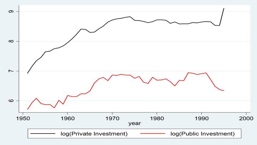
conversely, below the average in the subsequent phase (that is, when the Italian growth rate was
lower) (Felice and Vecchi, 2015b). This pattern of growth can be interpreted looking at the post-war
structural dynamics in the Mezzogiorno. Figure 3 shows trends of private and public investment that
are consistent with the trend of productivity presented in Figure 1.
 Throughout this period, a massive scheme of regional development was carried out by the Italian
state – the so-called «extraordinary intervention», mostly coinciding with the lifespan of the State-
owned agency «Cassa per il Mezzogiorno» (1950-1984) – which was generally regarded as effective
in the first part (from the 1950s to the early 1970s), ineffective and even damaging in the second
(from the early 1970s to the 1980s). In the first part of its life, the Cassa devoted most of its resources
to «direct interventions», which included general and sector-specific infrastructures (mostly
aqueducts, roads, drainage and agricultural settlements), plus other minor interventions (railroads,
school construction, education and professional training, development assistance, research and
development); from 1957 onwards, subsidies to entrepreneurs (grants to agriculture, tourism,
craftsmanship, fishing, but above all to industry) grew in importance, reaching about one third of total
expenditures from the mid-1960s to the mid-1970s (e.g. La Spina, 2003; Felice, 2007a; Felice and
Lepore, 2016). Therefore, the activity of the Cassa affected both public and private investments.
Overall, the total expenditures of the Cassa amounted to 0.69 of total Italian GDP in the years 1950-
1965, decreased to an average 0.64 in the years 1966-1970, rose again to an average 0.84 in the 1970s,
and then finally decreased to an average 0.61 in the early 1980s (Felice and Lepore, 2017). Although
in the 1970s the funds allocated through the Cassa reached their peak, however, they lost
effectiveness, having come to be strongly affected by political political pressure and nepotism, which
resulted into unproductive uses. In the same period, also the convergence of southern Italy came to a
halt, and never resumed.
 One question often raised in the literature on the effects of public capital on economic growth is
the direction of causation that could also be reversed. Indeed, although the decision to invest in
infrastructures is usually made by policy makers, it can be easily argued that as the wealth of a country
increases, more resources can be spent on public capital. In the context of the present study, the
exogeneity of public investment can be justified by important arguments. It is well known (e.g., Fauri,
2010; D’Antone, 1995; Lepore, 2012a, 2013 and 2016) that in the first phase of its reconstruction
after World War II Italy took advantage of the funds from international institutions and the USA. A
significant share of these resources was allocated to infrastructures in the Mezzogiorno. This is the
case of the financial aid of the World Bank to the Cassa per il Mezzogiorno in the 1950s and mid-
1960s, after which a large part of the resources for public investment in southern Italy came from the

national budget. In the empirical analysis, we test the hypothesis of the long-run causality between
public investments and GDP.

 3. Econometric model and results

The contribution of public capital to the process of economic development in the long-run is usually
modelled in the context of production functions. In this paper, we assume the aggregate output (Y)
depends on the state of technology (A) and three inputs - private capital (K), public capital ( ) and
labour (N) - according to the following Cobb-Douglas production function with constant returns to
scale:
 = 1− − . (1)
Taking logs on both sides of equation (1) yields the following equation:

 ln( ) = ln( ) + ln( ) + ln( ), (2)
where lowercase letters indicate variables in per worker terms.
 Equation (2) represents the basic model of our econometric analysis. In this framework, we
choose to approximate the two capital stock variables with investment data to for two reasons. The
first relates to the integration properties of the time series of investment and capital. Indeed, it can be
noted in the literature that aggregate capital is usually integrated of the second order, whereas
production and investment are integrated of order one (Everaert, 2003; Haldrup, 1998; Otto and Voss,
1996). Hence, the estimation of model (2) on data of stock variables could produce a “spurious
regression”. This econometric problem has been noted in several papers closely related to this paper
as Sturm et al., (1999); Pereira and Andraz, (2005); Herranz (2007), among others, where investment
substitutes for capital stock. The second reason refers to the lack of capital stock time series for
southern Italy on the period before 1970. Restricting the analysis to the years after 1969 would
preclude any statistical approach to structural change in the economic development of the
Mezzogiorno, which is one of the main objectives of this paper.
 The empirical analysis is conducted on time series of the Italian Mezzogiorno in the period
1951-1995. The economic variables included in model are Real Gross Domestic Product per unit of
labour (hereafter y) which is used as a measure of the economic performance, Real Gross fixed private
investments per unit of labour (hereafter priv_inv) and Real Gross fixed public investments per unit
of labor (hereafter pub_inv).

 3.1 Cointegration analysis
The econometric analysis is based on the following model:

log( ) = + ( _ ) + ( _ ) + . (3)

If the Data Generating Process (DGP) of the variables in equation (3) is characterized by a stochastic
trend, a cointegration analysis could show the existence of a long-run relationship that can be
interpreted as the causal explanation of productivity of the economy of southern Italy.
 Accordingly, preliminarily we test for stationarity and order of integration among all
variables. We run two unit-root tests: the augmented Dickey–Fuller (ADF) and the Phillips-Perron
(PP) test (Phillips and Perron 1988), for both the level and the first differences of all variables (see
Table 2). The null hypothesis of both tests is that the variable contains a unit root, and the alternative
is that the variable is generated by a stationary process with or without a deterministic trend.

Table 2. Augmented Dickey-Fuller and Phillips-Perron unit root tests
 Level First differences
 Variable ADF test PP test ADF test PP test
 log(y) -0.95 (0.94) -0.74 (0.96) -1.98 (0.02) -5.53 (0.00)
 log(priv_inv) -2.36 (0.40) -2.89 (0.16) -2.68 (0.00) -2.80 (0.05)
 log(pub_inv) -0.58 (0.97) -1.04 (0.93) -2.82 (0.00) -7.01 (0.00)
Note: p-values in parentheses. Two lags are used for both the tests. Results are robust to the variation of the lag length. In
both ADF and PP tests, the associated regression for all the variables in level contains a time trend.

The test statistics suggest the hypothesis of a unit root in the DGP cannot be rejected for the levels of
the three variables, while it can be rejected in the case of their first differences. Hence, the time series
are probably integrated of order one, I(1).
 In this case, one or two cointegrating equations could represent the long-run relationships
among the three variables. We apply the Johansen’s (1991) trace test to determine the number of
cointegrating equations in a Vector Error Correction Model (VECM) of the relationships among
log(y), log(pub_inv) and log(priv_inv). In the Johansen procedure, the VAR optimal lag length of one
year has been chosen by the standard information criteria.4 In the VECM we assume a linear trend in
the cointegrating relations.

Table 3. Johansen multivariate cointegration (CE) test

4
 Schwarz's Bayesian information criterion, and the Hannan and Quinn information criterion both indicate one lag
order for the VAR, while the Akaike's information criterion suggests a lag order of four. To save degrees of freedom we
choose one lag in our VECM. Cointegration analysis has been performed using STATA 14 statistical software.

Hypothesized
 No. of CE(s) Trace statistic 5% critical value
 None 46.26 42.44
 *
 At most 1 22.17 25.32
 At most 2 6.52 12.25
Note: the VAR lag length is one. * denotes acceptation of the null hypothesis at the 5% level.

The trace test statistics in Table 3 show we cannot reject the hypothesis of a cointegration rank of
one, indicating one cointegrating equation at the 0.05 level. Applying the Johansen’s (1992)
maximum likelihood estimation method to the VECM specified assuming one lag order and one
cointegrating relation provides the parameters of the long-run equation shown in Table 4.

Table 4. Cointegrating equation

Variable Coefficient Std. Error t-Statistic P-value
log(y) 1

log(pub_inv) -0.181 0.051 -3.54 0.00

log(priv_inv) -0.362 0.041 -8.76 0.00

trend -0.019 0.00 -17.42 0.00

constant -1.176

This equation can be interpreted as an estimate of model (3):
 log( ) = 1.176 + 0.019 + 0.181log( _ ) + 0.362 + log(priv_inv)

In order to complete the cointegration analysis, table 5 below shows the results of a Lagrange
multiplier test for the autocorrelation in the residuals of the VECM that we estimated. The null
hypothesis of the test is the absence of autocorrelation that we always accept when the test is
performed at lags from 1 to 5.

Table 5: Autocorrelation test

lag Chi2 df Prob > chi2
1 10.02 9 0.34
2 10.95 9 0.27
3 14.81 9 0.10
4 13.04 9 0.16
5 7.74 9 0.56

The estimates of the VECM provide further useful information over the long-run relationships among
the three variables, and are shown in Table 6. Because the VAR has one lag order, the VECM includes
the Error Correction Term (ECT) one year lagged, but does not include the short-run dynamics. The
adjustment coefficient of the equation for Δln(y) is negative and statistically significant with absolute
value lower than 1. The same coefficients in the other two equations are not statistically significant.
These results have useful implications for the interpretation of the estimated cointegrating equation
in terms of causal effects. Indeed, statistical inference suggests the ECT enters significantly the
equation of output per unit of labour, but does not contribute to the explanation of the two investment
variables. Hence, both variables can be considered weakly exogenous for the long-run cointegrating
equation.

Table 6. Adjustment coefficients in VECM estimates
 Coefficient t-Statistic P-value
Equation: Δln(y)
 −1 -0.25 -2.84 0.00

Equation: Δln(pub_inv)
 −1 0.54 1.21 0.22

Equation: Δln(priv_inv)
 −1 0.51 1.38 0.17

The application of the Johansen (1995) framework to cointegration analysis suggests the existence of
one equilibrium relationship where both public and business investment Granger cause in the long-
run the GDP per worker of southern Italy in the period after World War II. Both effects are
remarkable, but that of the private sector investments is greater (double) that that of government
investment.
 Since the same analysis supports the hypothesis of a single cointegrating equation, in the
following we will check the robustness of our results by estimating the equilibrium equation (3) using
two alternative methods: Fully Modified OLS (FMOLS) of Philips and Hansen (1990), and Dynamic
OLS (DOLS) proposed by Saikkonen, (1992) and Stock and Watson, (1993). The FMOLS estimator
corrects the single-equation estimates for simultaneity bias and residual autocorrelation that affect
OLS in small samples. The same correction is obtained by the DOLS estimator by adding the leads
and lags of the first difference of the regressors in the cointegrating equation. Table 7 presents the
results of the estimation of equation (3) with both methods.5 Overall, the estimates confirm the results
we have obtained applying the Johansen’s framework. In this single-equation approach the hypothesis

5
 We performed FMOLS and DOLS estimates using the STATA unofficial command cointreg by Wang and Wu (2012).

of cointegration can be tested by performing a test of stationarity of the error correction term derived
from FMOLS and DOLS estimates. Table 7 presents the KPSS (Kwiatkowski et al., 1992) test
statistic that shows the null hypothesis of stationary residuals cannot be rejected.
 The results of the cointegration analysis of model (3) highlight the fundamental role that both
public and business capital accumulation played in the process of development of southern Italy in
the period 1951-1995. The private sector seems to lead economic growth with the important
contribution of state investments in infrastructures. The statistically significant parameter of a linear
trend suggests the Mezzogiorno economy grew following a virtuous circle involving physical capital
accumulation and technical progress. This picture is coherent with that offered by the literature on
the economic history of Italy, where, however, great emphasis is put on two main phases of the
process of development in the post-war era, as already argued above in this paper. One of the main
hypothesis advanced in the literature ascribes the transition from the “golden age” to the recent low
growth period to the lower efficacy of the government structural policies occurred starting with the
“oil crisis”. In the following, we will investigate structural change in the Mezzogiorno economy with
the instruments offered by dynamic econometric analysis.

Table 7. Dependent variable: Real GDP per unit of labour. FMOLS and DOLS estimates.

 (1) (2)
 FMOLS DOLS

 ln(pub_inv) 0.117*** 0.167**
 (2.887) (2.442)

 ln(priv_inv) 0.390*** 0.352***
 (10.267) (6.256)

 trend 0.021*** 0.020***
 (20.321) (15.269)

 Observations 44 42
 KPSS on residuals 0.231 0.328
 KPSS 5% critical value 0.463 0.463
 R2 0.993 0.996
Note. The lead and lag order in DOLS is 1 t statistics in parentheses. The KPSS statistic tests the null hypothesis that the residuals of the regression
are stationary; the maximum lag has been chosen by Schwert criterion; the long-run variance of the time series has been calculated using the
Quadratic Spectral kernel. * p < 0.10, ** p < 0.05, *** p < 0.01.

 3.2 Structural change in the post-war process of development of southern Italy
 The bar chart of the time series of the growth rate of real GDP per worker in southern Italy (Figure
2) shows clear evidence of a break in the early 1970s. Indeed, the average growth performance seems
to decrease after the first three decades following the end of World War II. This has been widely

reported by those concerned with the effects of government policy on development in the
Mezzogiorno. A widely accepted explanation relates it to a less effective (and progressively lower)
State involvement in public capital formation and in providing incentives for industrialisation
(Barbagallo and Bruno, 1997; Cafiero, 2000; Felice, 2013; Lepore, 2013; Felice and Lepore, 2016).
Given the relevance of this issue to the debate and the aim of this paper, we search for statistical
evidence that would corroborate the hypothesis that economic growth in the Mezzogiorno after World
War II has been characterized by two regimes. Our strategy first searches for the presence and number
of breaks in the time series of the southern Italy’s growth rate, then concentrates on structural change
in the model of economic growth, focusing on the role of capital (public and private) accumulation.

 3.2.1 Breaks in the time series of the growth rate of GDP per worker
 In this section, we search for breaks in the growth rate of GDP per unit of labour in the period
1951-1995. We apply the methodology proposed by Bai and Perron (1998; 2003a) that allows a
general modelling framework to determine multiple breakpoints in Δ . Accordingly, we assume the
variable Δ follows the model:
 Δ = + , = 1, … … . , (2)
where t is a time index and is the random disturbance that can be autocorrelated and
heteroscedastic. Structural change in model (2) means the parameter changes because of m breaks:
 Δ = + , = −1 + 1, … … . , = 1, … , + 1 (3)

where denotes the regime, and the convention that 0 = 0 and +1 = is used. According to
model (3), the time series of value added per worker can be subject to m changes of the drift parameter
 . This econometric model presents two fundamental questions. The first is the determination of m.
The second is the estimation of the parameter in each regime, and the estimation of the unknown
break points .
 Bai and Perron (1998) propose three tests of structural change. The first, ( ), tests the null
of no structural break versus the alternative of m=k breaks. The second, called Double Maximum
Test, refers to the same null hypothesis against the alternative of an unknown number of breaks given
an upper bound M. Two versions of the test statistic are proposed: UDmax and WDmax. The third,
 ( + 1| ), can be applied to a sequence of tests for l versus l+1 breaks. All these tests allow for
serially correlated errors and different distributions for the time series and the errors across regimes.
Since these tests do not have a standard distribution, Bai and Perron (1998; 2003b) provide simulated
critical values. The whole framework is based on the objective of minimising the sum of squared
residuals of the model (3). This optimisation problem is constrained by the restriction that the

segments between two break points define regimes with a minimum length, h. This constraint has a
technical justification (see Bai and Perron, 1998; 2003a) but is also consistent with intuition and
econometric practice.6
 Table 8 presents the results of the application of this procedure to the time series of the rate of
growth of productivity in southern Italy. We allow up to three breaks and assume a trimming
percentage of 20%, which implies regimes with minimum length of nine years. Equation (3) is
estimated under the assumption of heteroskesdasticity and serial correlation of the error in each
 7
regime. The three tests suggest the rejection of the null of no structural change in favour of the
alternative of one break, at a 1% significance level. The procedure also provides the estimate of the
year in which structural change occurs: 1974. The estimated parameters of equation (3) are: =
0.053 ( = 12.37) for the years 1952-1973; = 0.016 ( = 3.90) for the years 1974-1995.

Table 8. Bai-Perron tests of structural change
 Test Statistic Value Critical Value
 supFT(1) 46.31*** 11.94
 supFT(2) 24.60*** 8.77
 supFT(3) 13.11*** 6.58
 UDmax 46.31*** 12.02
 WDmax 46.31*** 13.16
 supFT(1|0) 46.31*** 11.94
 supFT(2|1) 3.91 13.61
Note: Critical values from Bai and Perron, 2003b. *** Significance at the 1% level.

 3.2.2 Structural change in the model of economic growth
In this section, we investigate structural change in the long-run relationship between public and
private investment and output per worker taking into account the results of the Bai-Perron tests. We
follow the approach proposed by Hansen (1992) to test the stability of cointegrated regression models.
As in Hansen (1992), the estimation method is the fully modified OLS. When the break date is known,
the F statistic of Hansen (1992) – that corresponds to the classical Chow test - can be used to test the
null hypothesis the parameters of the regression equation do not change. If the timing of the break is
unknown, the SupF test statistic can be used to test the same null hypothesis. In this case, the sequence
of F statistic is calculated for every break year in a subsample derived after the trimming of a share
of the first and last observations. In both cases, if the test rejects the null, the alternative is one break

6
 The optimization problem described above implies complex computations that Bai and Perron simplify by proposing a
sequential algorithm based on dynamic programming. We performed all computations using Eviews 8.1.
7
 Andrews's framework (1991) is followed to construct a covariance matrix consistent to heteroscedasticity and
autocorrelation using a quadratic spectral kernel and the "pre-whitening" of the residuals with a VAR(1) model.

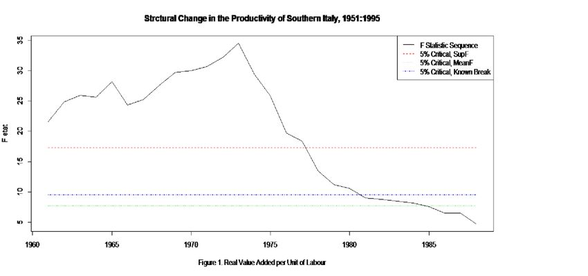
in the parameters. The other two statistics proposed by Hansen – MeanF and – test the same null
hypothesis, but under the alternative hypothesis both assume the parameters can be modelled as a
martingale process.

Table 9. Tests for Parameter Stability

 Test Statistic P-value Critical value at 5%

 SupF 34.548 0.01 17.3

 MeanF 19.596 0.01 7.69

 1.995 0.01 0.778

Note. P-values and asymptotic critical values from Hansen (1992).

 The results of the application of the Hansen’s (1992)8 testing procedure to the cointegrating
equation that we estimated in the previous section, are shown in Table 9. The three statistics take
values much bigger than the 5% critical values. Figure 4 displays the line of the sequence of F
statistics that lies above the 5% SupF critical value for a large part of the period, and presents its
largest value in 1974. Hence, this testing methods for integrated I(1) time series are consistent with
those of Bai and Perron (1998) because both suggest that one structural break in the process of
economic growth of southern Italy occurred in 1974.
 We investigate structural change with the estimation of two distinct models on data of the first
regime, 1951-1973, and of the second, 1974-1995. The application of FMOLS to the time series of
the two periods provides two really different equations displayed in Table 10. In both regressions,
KPSS test suggests the level stationarity of the error-correction term in the VECM of the three
variables, which means they are cointegrated.

Table 10. Dependent variable: Real GDP per unit of labour. FMOLS estimates.

 (1) (2)

 1951-1973 1974-1995

8
 All the calculations have been performed using the R programs of Bruce Hansen, available at his homepage:
http://www.ssc.wisc.edu/~bhansen/progs/jbes_92.html. The trimming region of the time series is [0.2, 0.8].

ln(pub_inv) 0.197*** 0.011
 (5.510) (0.348)

 ln(priv_inv) 0.152*** 0.082*
 (2.821) (1.752)

 trend 0.033*** 0.016***
 (5.977) (18.135)

 Observations 22 21
 KPSS on residuals 0.132 0.104
 KPSS 5% critical value 0.463 0.463
 R2 0.993 0.958
Note. t statistics in parentheses. The KPSS statistic tests the null hypothesis that the residuals of the regression are
stationary; the maximum lag has been chosen by Schwert criterion; the long-run variance of the time series has been
calculated using the Quadratic Spectral kernel. * p < 0.10, ** p < 0.05, *** p < 0.01.

In the first equation, the estimates of the parameters of public and private investment are positive and
strongly statistically significant. The State intervention on infrastructures seem to lead the growth
process in the first two decades after World War II: the long-run elasticity of output to public
investment is close to 20%, although the private sector shows a comparable contribution to growth.
The picture changes dramatically under the second regime, 1974-1995. Indeed, estimates highlight
how in the period public capital accumulation strongly loses efficacy – the parameter is not
statistically significant – while productivity increases because of private investment, whose parameter
is significant but half of that of post-war years. The estimates of the trend parameter seem coherent
with the general impression given by the two equations. Indeed, they are both significant and positive
with a value in the first equation double than that in the second equation. The overall picture that
comes out of the cointegration analysis tells of a period of sustained growth of southern Italy in the
first two post-war decades that is driven by all the main components of long-term growth: public
infrastructure, business investment, and technical progress. In the early seventies, the economic crisis
hits Italy as most of the world. Our regression analysis suggests in southern Italy the crisis means
strong inefficiency of State intervention and serious difficulties in the business sector.

 4. Concluding remarks
 The article estimates for the first time the contribution of public and private investments to the
economic growth of southern Italy in the second half of the twentieth century (1951-1996). The forty-
five years under scrutiny can be divided into two different periods: in the first (1951-1973) the growth
of per capita GDP in southern Italy was considerably higher, to the extent that those decades were
also the only ones, in the entire history of post-unification Italy, when southern Italy managed to
converge to the Italian average (Lepore, 2012b; Felice and Vecchi, 2015b); in the years 1974-1996,

conversely, the growth rate of per capita GDP was lower, and even the convergence of southern Italy
came to a halt (even though Italy as a whole was also growing at a much slower pace than before)
(Toniolo, 2013; Felice, 2015b). In order to analyse the contribution of public and private investments
to GDP growth, we estimate a dynamic econometric model on annual time series of the Mezzogiorno
economy. In this model, the main explanatory variables are public and private investments.
 Our results confirm, for the first time on quantitative grounds, the important role played by public
investments for the economic growth of southern Italy, and are in line with hypotheses put forward
by previous historical and qualitative studies (Del Monte and Giannola, 1978; Felice and Lepore,
2016). The econometric analysis of structural change in the economic performance of the
Mezzogiorno produces, for the first time in the literature, the estimates of two distinct models of
growth before and after the year 1974. In the first period, all the main determinants of economic
growth seem to drive southern Italy out of underdevelopment. In this process, state intervention on
infrastructures is the leading factor. The same estimates show the dramatic change in the process of
growth started with the oil crisis. The main finding of this analysis is the irrelevant effect of structural
public policy on the economic performance of the Mezzogiorno, that relied on investments of the
business sector.
 This broad result has a further, important qualification. When running structural breaks, we
observe that there are relevant differences in the effect of public investments between the two periods:
it was positive in the first period (1951-1973), not significant in the second (1974-1995). This too is
an important finding, confirming on aggregate and econometric terms what a vast literature, based on
case studies or from qualitative grounds, has also maintained: that public intervention was effective
only during the “golden age”, while from the 1970s onward it lost its effectiveness due to
misallocations and unproductive uses. This conclusion has been put forward with particular reference
to the Cassa per il Mezzogiorno, which among other things played a significant role in public
investments especially in the first period (Felice and Lepore, 2017); now, it is confirmed also for
public intervention as a whole.

 Our results have important implications also beyond academia, for policy makers, especially
when considered together with the main findings from historical or qualitative analyses about public
intervention in southern Italy. The main conclusion to be drawn is that public investments can either
be positive, ineffectual or even negative for economic growth, crucially depending on the way they
are made and the macro-economic setting they operate in. More specifically for Italy, the literature
on public intervention and the economic history of the Mezzogiorno in the second half of the twentieth
century (e.g. Trigilia, 1992; Felice, 2007a; Felice and Lepore, 2017) provide useful insights not only

into the preconditions for success during the economic miracle – impermeability to clientelistic
pressures, separation from and complementariness to ordinary administration, consistency with an
encompassing development strategy based on infrastructures and industry – but also into the reasons
behind the subsequent ineffectiveness or even counter-productiveness; to these, we had that a further
reason could be the decline of extraordinary interventions in favour of ordinary ones. Long-run
econometric analyses proposed for other countries, such as that on the role of infrastructural
investments for Spain (1850-1935), also confirm that the impact of public intervention may
significantly vary according to typology and allocation criteria (Herranz-Loncán, 2007).
 It goes without saying that further research would be invaluable in order to corroborate or qualify
our findings. At a higher territorial breakdown, it would be possible to replicate the econometric
analyses for each region in southern Italy, following recent economic history studies which have
pointed out significant differences in the qualities and strategies of public intervention in the second
half of the twentieth century (Felice, 2007b; Felice, Lepore and Palermo, 2015b), as well as in the
patterns of economic growth among the southern regions.

References
 Abramovitz, M. (1986). Catching up, forging ahead and falling behind. Journal of Economic
History, 46 (2), 385-406.
 Acconcia, A., and A. Del Monte. "Le politiche per il rilancio dello sviluppo del Mezzogiorno."
Il Mulino (2000).
 Andrews, D.W.K. (1991). Heteroscedasticity and autocorrelation consistent covariance matrix
estimation. Econometrica, 59, 817-858.
 Bai, J., and P. Perron (1998). Estimating and testing linear models with multiple structural
changes. Econometrica, 66(1), 47-78.
 Bai, J., and P. Perron (2003a). Computation and analysis of multiple structural change models.
Journal of applied econometrics, 18(1), 1-22.
 Bai, J., and P. Perron (2003b). Critical values for multiple structural change tests. The
Econometrics Journal, 6(1), 72-78.
 Banfield, E. (1958). The Moral Basis of a Backward Society. Free Press: New York.
 Barbagallo, F., and G. Bruno (1997). Espansione e deriva del Mezzogiorno. In F. Barbagallo,
ed., Storia dell’Italia repubblicana, vol. III. L’Italia nella crisi dell’ultimo ventennio. 2. Istituzioni,
politiche, culture. Einaudi: Turin, 399-470.
 Barca Barca, F. (2006). Italia frenata. Paradossi e lezioni della politica per lo sviluppo. Donzelli:
Rome.
 Barro RJ, Sala-i-Martin X. 1992. Public finance in models of economic growth. Review of
Economic Studies, 59(4) 645-661.
 Barro, R.J. (1990). Government spending in a simple model of endogenous growth. Journal of
Political Economy, 98, S103–S125.
 Barro, R.J. (1991). Economic growth in a cross section of countries. Quarterly Journal of
Economics, 106, 407-443.
 Barro, R.J. (1996). Determinants of economic growth: a cross-country empirical study. NBER
Working Paper, 5698.
 Battilossi, S., Foreman-Peck, J., and G. Kling (2010). Business cycles and economic policy,
1945–2007. In S. Broadberry and K.H. O’Rourke, eds., The Cambridge Economic History of Modern
Europe. Volume 2. 1870 to the Present. Cambridge University Press: Cambridge, 360-389.
 Baum, Christopher F., Mark E. Schaffer, and Steven Stillman. (2007) "Enhanced routines for
instrumental variables/GMM estimation and testing." Stata Journal, 7.4: 465-506.
 Baumol, W.J. (1986). Productivity growth, convergence and welfare: what the long-run data
show. American Economic Review, 76(5), 1072-85.

Bevilacqua, P. (1993). Breve storia dell’Italia meridionale dall’Ottocento a oggi. Donzelli:
Rome.
 Blomstrom, M., Lipsey, R.E., and M. Zejan (1996). Is Fixed Investment the Key to Economic
Growth? Quarterly Journal of Economics, 111, 269-276.
 Boltho, A. (2013). Italy, Germany, Japan: From Economic Miracles to Virtual Stagnation. In G.
Toniolo, ed., The Oxford Handbook of the Italian Economy since Unification. Oxford University
Press: Oxford, 108-133.
 Bom, P. R., & Ligthart, J. E. (2014). What have we learned from three decades of research on the
productivity of public capital?. Journal of economic surveys, 28(5), 889-916.
 Bonaglia, Federico, Eliana La Ferrara, and Massimiliano Marcellino. "Public capital and
economic performance: evidence from Italy." Giornale degli Economisti e Annali di Economia
(2000): 221-244.
 Bronzini, Raffaello, and Paolo Piselli. "Determinants of long-run regional productivity: the role
of R&D, human capital and public infrastructure." (2006).
 Cafiero, S. (1996). Questione meridionale e unità nazionale (1861-1995). La Nuova Italia
Scientifica: Rome.
 Cafiero, S. (2000). Storia dell’intervento straordinario nel Mezzogiorno (1950-1993). P. Lacaita:
Manduria, TA.
 Carey, J.P.C., and A.G. Carey (1955). The South of Italy and the Cassa per il Mezzogiorno. The
Western Political Quarterly, 8 (4), 569–588.
 Carlyle, M. (1962). The Awakening of Southern Italy. Oxford University Press: Oxford.
 Caselli, F., Esquivel, G., and F. Lefort (1996). Reopening the Convergence Debate: A New Look
at Cross-Country Growth Empirics. Journal of Economic Growth, 1(3), 363-389.
 Crafts, N., and G. Toniolo (2010). Aggregate growth, 1950–2005. In S. Broadberry and K.H.
O’Rourke, eds., The Cambridge Economic History of Modern Europe. Volume 2. 1870 to the Present.
Cambridge University Press: Cambridge, 296-332.
 Cumby, R.E., and J. Huizinga (1990). Testing the autocorrelation structure of disturbances in
ordinary least squares and instrumental variables regressions. NBER Technical Working Paper, No.
92.
 Cumby, R.E., and J. Huizinga (1992). Testing the autocorrelation structure of disturbances in
ordinary least squares and instrumental variables regressions. Econometrica, 60(1), 185-195.
 D’Antone, L. (1995). L’«interesse straordinario» per il Mezzogiorno (1943-1960). Meridiana,
9(24), 17-64.
 Daniele, V., and P. Malanima (2007). Il prodotto delle regioni e il divario Nord–Sud in Italia
(1861–2004). Rivista di Politica Economica, 97(2), 267-315.

De Long, J.B., and L. Summers (1991). Equipment Investment and Economic Growth. Quarterly
Journal of Economics, 106(2), 445-502.
 De Long, J.B., and L. Summers (1993). How Strongly do Developing Economies Benefit from
Equipment Investment? Journal of Monetary Economics, 32(3), 395-415.
 Del Monte, A., and A. Giannola (1978). Il Mezzogiorno nell’economia italiana. Il Mulino:
Bologna.
 Durlauf, S.N., Johnson, P.A., and J.R.W. Temple (2005). Growth Econometrics. In P. Aghion
and S.N. Durlauf, eds. Handbook of Economic Growth, Vol. 1A. North-Holland: Amsterdam, 555-
677.
 Easterly, W., and S. Rebelo (1993). Fiscal Policy and Economic Growth: An Empirical
Investigation. Journal of Monetary Economics, 32(3), 417-458.
 Engle, Robert F., and Clive WJ Granger. "Co-integration and error correction: representation,
estimation, and testing." Econometrica: journal of the Econometric Society (1987): 251-276.
 Everaert, G. (2003). Balanced growth and public capital: an empirical analysis with I (2) trends
in capital stock data. Economic Modelling, 20(4), 741-763.
 Fauri, F. (2010). Il piano Marshall e l’Italia. Il Mulino: Bologna.
 Felice, E. (2005). Il valore aggiunto regionale. Una stima per il 1891 e per il 1911 e alcune
elaborazioni di lungo periodo (1891-1971). Rivista di Storia Economica, 21(3), 83-124.
 Felice, E. (2007a). Divari regionali e intervento pubblico. Per una rilettura dello sviluppo in
Italia. Il Mulino: Bologna.
 Felice, E. (2007b). The «Cassa per il Mezzogiorno» in the Abruzzi. A successful regional
economic policy. Global & Local Economic Review, 10, 9-33.
 Felice, E. (2010). State Ownership and International Competitiveness: the Italian Finmeccanica
from Alfa Romeo to Aerospace and Defence. Enterprise and Society, 11(3), 594-635.
 Felice, E. (2012). Regional convergence in Italy (1891-2001): testing human and social capital.
Cliometrica, 6(3), 267-306.
 Felice, E. (2013). Perché il Sud è rimasto indietro. Il Mulino: Bologna.
 Felice, E. (2015a). La stima e l’interpretazione dei divari regionali nel lungo periodo: i risultati
principali e alcune tracce di ricerca. Scienze Regionali / Italian Journal of Regional Science, 14(3),
91-120.
 Felice, E. (2015b). Ascesa e declino. Storia economica d’Italia. Il Mulino: Bologna.
 Felice, E., and A. Lepore (2016). State intervention and economic growth in Southern Italy: the
rise and fall of the «Cassa per il Mezzogiorno» (1950-1986). Business History, in press.
http://dx.doi.org/10.1080/00076791.2016.1174214

Felice, E., and G. Vecchi (2015a). Italy’s Modern Economic Growth, 1861-2011. Enterprise and
Society, 16(2), 225-248.
 Felice, E., and G. Vecchi (2015b). Italy’s Growth and Decline, 1861-2011. Journal of
Interdisciplinary History, 45(4), 507-548.
 Felice, E., and M. Vasta (2015). Passive Modernization? The New Human Development Index
and its Components in Italy’s Regions (1871-2007). European Review of Economic History, 19(1),
44-66.
 Felice, E., Lepore, A., and S. Palermo (2015b). La dimensione regionale dell’intervento
straordinario per il Mezzogiorno. In E. Felice, A. Lepore, S. Palermo, eds., La convergenza possibile.
Strategie e strumenti della Cassa per il Mezzogiorno nel secondo Novecento. Il Mulino: Bologna,
149-188.
 Felice, E., Lepore, A., and S. Palermo, eds. (2015a). La convergenza possibile. Strategie e
strumenti della Cassa per il Mezzogiorno nel secondo Novecento. Il Mulino: Bologna.
 Felice, E., and A. Lepore (2017). State intervention and economic growth in Southern Italy: the
rise and fall of the ‘Cassa per il Mezzogiorno’ (1950-1986). Business History, 59(3), 319-341.
 Gallup, J.L, Sachs, J.D., and A.D. Mellinger (1998). Geography and Economic Development.
NBER Working Paper, No. w6849, National Bureau of Economic Research.
 Glomm, G., and B. Ravikumar (1994). Public investment in infrastructure in a simple growth
model. Journal of Economic Dynamics and Control, 18, 1173-1187.
 Glomm, G., and B. Ravikumar (1998). Flat-Rate Taxes, Government Spending on Education,
and Growth. Review of Economic Dynamics, 1(1), 306-325.
 Haldrup, Niels. "An econometric analysis of I (2) variables." Journal of Economic Surveys 12.5
(1998): 595-650.
 Hansen, B. E. (1992). Tests for parameter instability in regressions with I(1) processes. Journal
of Business & Economic Statistics, 10(3), 321-335.
 Herranz-Loncán, A. (2007). Infrastructure investment and Spanish economic growth, 1850–
1935. Explorations in Economic History, 44, 452-468.
 Islam, N. (1995). Growth Empirics: A Panel Data Approach. Quarterly Journal of Economics,
110(4), 1127-1170.
 Johansen, S., 1991. Estimation and hypothesis testing of cointegrating vectors in Gaussian vector
autoregressive models. Econometrica 59, 1551_1580.
 Kwiatkowski D., Phillips P. C., Schmidt P., Shin Y. (1992). Testing the null hypothesis of
stationarity against the alternative of a unit root: How sure are we that economic time series have a
unit root?. Journal of Econometrics, 54(1-3), 159-178.

La Ferrara, E., and M. Marcellino. (1999). "TFP, Costs, and Infrastructure: An Equivocal
Relationship."
 La Spina, A. (2003). La politica per il Mezzogiorno. Il Mulino: Bologna.
 Lepore, A. (1991). La questione meridionale prima dell’intervento straordinario. Lacaita:
Manduria.
 Lepore, A. (2011a). Il dilemma del Mezzogiorno a 150 anni dall’unificazione: attualità e storia
del nuovo meridionalismo. Rivista Economica del Mezzogiorno, 1-2, 57-90.
 Lepore, A. (2011b). La valutazione dell’operato della Cassa per il Mezzogiorno e il suo ruolo
strategico per lo sviluppo del Paese. Rivista Giuridica del Mezzogiorno, 1-2, 281-317.
 Lepore, A. (2012a). Cassa per il Mezzogiorno e politiche per lo sviluppo. In A. Leonardi, ed.,
Istituzioni ed Economia, Cacucci: Bari.
 Lepore, A. (2012b). Il divario Nord-Sud dalle origini a oggi. Evoluzione storica e profili
economici. In M. Pellegrini, ed., Elementi di diritto pubblico dell’economia, Cedam: Padova, 347-
367.
 Lepore, A. (2013). La Cassa per il Mezzogiorno e la Banca Mondiale. Un modello per lo sviluppo
economico italiano. Rubbettino: Soveria Mannelli, CZ.
 Lepore, A. (2015). La Cassa per il Mezzogiorno e lo sviluppo economico italiano: una
rivisitazione di lungo periodo, dalla golden age a oggi. In SVIMEZ, ed., La dinamica economica del
Mezzogiorno dal secondo dopoguerra alla conclusione dell’intervento straordinario. Il Mulino:
Bologna, 145-160.
 Lepore, A. (2016b). Questione meridionale e Cassa per il Mezzogiorno. In S. Cassese, ed.,
Lezioni sul meridionalismo. Nord e Sud nella storia d’Italia. Bologna: Il Mulino, 233-260.
 Levine, R., and D. Renelt (1992). A Sensitivity Analysis of Cross-Country Growth Regressions.
American Economic Review, 82(4), 942-963.
 Levine, R., and S. Zervos (1993). What We Have Learned About Policy and Growth from Cross-
Country Regressions, American Economic Review, 83(5), 426-430.
 Levine, Ross, and David Renelt. “A Sensitivity Analysis of Cross-Country Growth Regressions.”
The American Economic Review, vol. 82, no. 4, 1992, pp. 942–963. JSTOR,
www.jstor.org/stable/2117352.
 Lindahl, Mikael, and Alan B. Krueger. "Education for Growth: Why and for Whom?." Journal
of Economic Literature 39.4 (2001): 1101-1136.
 Lucas, R.E. (1988). On the mechanics of economic development. Journal of Monetary
Economics, 22, 3-42.

Mankiw, G.N., Romer, D. and D.N. Weil (1992). A Contribution to the Empirics of Economic
Growth. Quarterly Journal of Economics. 107(2), 407-437.
 Otto, Glenn D., and Graham M. Voss. "Public capital and private production in Australia."
Southern Economic Journal (1996): 723-738.
 Pereira, Alfredo M., and Jorge M. Andraz. "Public investment in transportation infrastructure
and economic performance in Portugal." Review of Development Economics 9.2 (2005): 177-196.
 Perron, P. (2006). Dealing with structural breaks. In H. Hassani, T.C. Mills and K.D. Patterson,
eds., Palgrave handbook of econometrics. Volume I: Econometric Theory. Palgrave Macmillan:
London, 278-352.
 Phillips, Peter CB, and Bruce E. Hansen. "Statistical inference in instrumental variables
regression with I (1) processes." The Review of Economic Studies 57.1 (1990): 99-125.
 Phillips, Peter CB, and Pierre Perron. "Testing for a unit root in time series regression."
Biometrika 75.2 (1988): 335-346.
 Picci L. (1999), Productivity and infrastructure in the Italian Regions, Giornale degli Economisti
e Annali di Economia, Vol. 58 (Anno 112), No. 3/4 (Dicembre 1999), pp. 329-353
 Picci, L., (1997), Infrastrutture e produttività: il caso italiano, Rivista di Politica Economica, 1.
 Prota, F., and G. Viesti (2012). Senza Cassa. Le politiche di sviluppo del Mezzogiorno dopo
l’intervento straordinario. Il Mulino: Bologna.
 Putnam, R.D. (1993). Making Democracy Work: Civic Traditions in Modern Italy, with R.
Leonardi and R.Y. Nanetti. Princeton University Press: Princeton, NJ.
 Romp, W., and J. de Haan (2007). Public Capital and Economic Growth: A Critical Survey.
Perspektiven der Wirtschaftspolitik, 8, 6-52.Rukhsana Kalim and Mohammad Shahbaz, (2008),
"Remittances and Poverty Nexus: Evidence from Pakistan", Oxford Business & Economics
Conference Program.
 Saikkonen, Pentti. "Estimation and testing of cointegrated systems by an autoregressive
approximation." Econometric theory 8.1 (1992): 1-27.
 Solow, R.M. (1956). A contribution to the theory of economic growth. Quarterly Journal of
Economics, 70(1), 65-94.
 Staiger, D., and J.H. Stock (1997). Instrumental variables regression with weak instruments.
Econometrica, 65, 557-586.
 Stock, J.H., and M. Yogo (2005). Testing for Weak Instruments in Linear IV Regression. In D.W.
Andrews and J.H. Stock, eds., Identification and Inference for Econometric Models: Essays in Honor
of Thomas Rothenberg. Cambridge University Press: Cambridge, 80-108.
 Stock, James H., and Mark W. Watson. "A simple estimator of cointegrating vectors in higher

order integrated systems." Econometrica: Journal of the Econometric Society (1993): 783-820.
 Sturm, Jan-Egbert, Jan Jacobs, and Peter Groote. "Output effects of infrastructure investment in
the Netherlands, 1853–1913." Journal of Macroeconomics 21.2 (1999): 355-380.
 Summers, R., and A. Heston (1991). The Penn World Table: An expanded set of international
comparisons, 1950-1988. Quarterly Journal of Economics, CVI, 327-368.
 SVIMEZ (1985) La formazione e l’impiego delle risorse e dell’occupazione del Mezzogiorno e
del Centro-Nord dal 1951 al 1983. Studi SVIMEZ. Estratto N. 26 – Nuova Serie, Anno XXXVIII –
N. 1 – gennaio-marzo.
 SVIMEZ (2011). 150 anni di statistiche italiane: Nord e Sud 1861-2011, edited by A. Giannola,
A. Lepore, R. Padovani, L. Bianchi e D. Miotti. Il Mulino: Bologna.
 Swan, T.W. (1956). Economic growth and capital accumulation. Economic Record, 32(2), 334-
361.
 Toniolo, G. (2013). An Overview of Italy’s Economic Growth. In G. Toniolo, ed., The Oxford
Handbook of the Italian Economy since Unification. Oxford University Press: Oxford, 3-36.
 Trigilia, C. (1992). Sviluppo senza autonomia. Effetti perversi delle politiche nel Mezzogiorno.
Il Mulino: Bologna.
 Vecchi, G., ed. (2011). In ricchezza e in povertà. Il benessere degli italiani dall’Unità a oggi. Il
Mulino: Bologna.
 Wang Q., and Wu N., (2012). Long-run covariance and its applications in cointegration
regression. The Stata Journal 12, Number 3, pp. 515–542.