Rendezvous in Cis-Lunar Space near Rectilinear Halo Orbit: Dynamics and Control Issues
←
→
Page content transcription
If your browser does not render page correctly, please read the page content below
aerospace
Article
Rendezvous in Cis-Lunar Space near Rectilinear Halo Orbit:
Dynamics and Control Issues
Giordana Bucchioni † and Mario Innocenti *,†

                                          Department of Information Engineering, University of Pisa, 56126 Pisa, Italy; giordana.bucchioni@hotmail.it
                                          * Correspondence: mario.innocenti@unipi.it
                                          † These authors contributed equally to this work.

                                          Abstract: The paper presents the development of a fully-safe, automatic rendezvous strategy between
                                          a passive vehicle and an active one orbiting around the Earth–Moon L2 Lagrangian point. This is
                                          one of the critical phases of future missions to permanently return to the Moon, which are of interest
                                          to the majority of space organizations. The first step in the study is the derivation of a suitable full
                                          6-DOF relative motion model in the Local Vertical Local Horizontal reference frame, most suitable
                                          for the design of the guidance. The main dynamic model is approximated using both the elliptic and
                                          circular three-body motion, due to the contribution of Earth and Moon gravity. A rather detailed
                                          set of sensors and actuator dynamics was also implemented in order to ensure the reliability of the
                                          guidance algorithms. The selection of guidance and control is presented, and evaluated using a
                                          sample scenario as described by ESA’s HERACLES program. The safety, in particular the passive
                                          safety, concept is introduced and different techniques to guarantee it are discussed that exploit the
                                          ideas of stable and unstable manifolds to intrinsically guarantee some properties at each hold-point,
                                in which the rendezvous trajectory is divided. Finally, the rendezvous dynamics are validated using

                                          available Ephemeris models in order to verify the validity of the results and their limitations for
Citation: Bucchioni, G.; Innocenti, M.
                                          future more detailed design.
Rendezvous in Cis-Lunar Space near
Rectilinear Halo Orbit: Dynamics and
                                          Keywords: rendezvous; NRHO; three-body problem
Control Issues. Aerospace 2021, 8, 68.
https://doi.org/10.3390/aerospace
8030068

Academic Editor: Vladimir S.
                                          1. Introduction
Aslanov                                         The paper presents some of the dynamics models and potential guidance algorithms
                                          usable for the preliminary assessment of a rendezvous between an unmanned vehicle
Received: 18 January 2021                 ascending from the Moon, and a permanent manned/unmanned service station located in
Accepted: 26 February 2021                a collinear Lagrangian point orbit of the Earth–Moon system. The motivation for this work
Published: 8 March 2021                   is given by the renewed interest of many government agencies and private organizations
                                          in returning to our satellite.
Publisher’s Note: MDPI stays neutral            The positive aspects of one such parking orbit lie in the possibility of continuous
with regard to jurisdictional claims in   communications with Earth, the visibility of the lunar hidden surface, and the relative low
published maps and institutional affil-   cost of station keeping maneuvers. Lagrangian points are known to be equilibria within a
iations.                                  circular restricted three-body model. Although the model is an approximation of the real
                                          multibody dynamics, it serves for a useful series of analyses, in particular when it comes
                                          to guidance and control algorithms, which, by nature, need simplified modeling for their
                                          primary design.
Copyright: © 2021 by the authors.               The attractiveness of the above orbits (Lissajous, halo, etc.) has been exploited over the
Licensee MDPI, Basel, Switzerland.        years by several missions, especially in the Sun–Earth system. The Solar and Heliospheric
This article is an open access article    Observatory and the Deep Space Climate Observatory are located at the L1 collinear point,
distributed under the terms and           while the Wilkinson Microwave Anisotropy Probe and the Gaia spacecraft used the L2
conditions of the Creative Commons        collinear point. The orbit of the James Webb telescope will be also located at the latter.
Attribution (CC BY) license (https://
                                                While the previous examples focused on science experiments and scientific knowledge,
creativecommons.org/licenses/by/
                                          the use of Lagrangian points in the Earth–Moon system is also considered for future human
4.0/).

Aerospace 2021, 8, 68. https://doi.org/10.3390/aerospace8030068                                            https://www.mdpi.com/journal/aerospace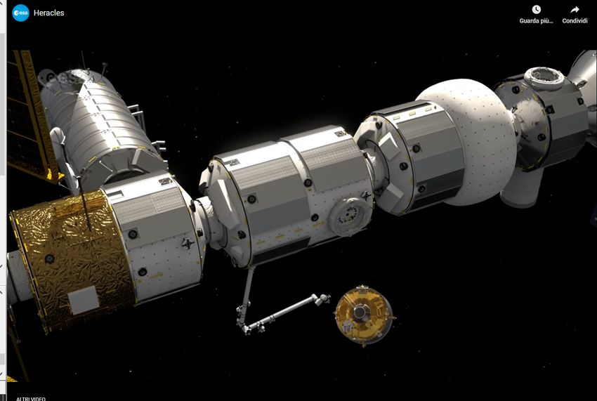
Aerospace 2021, 8, 68 2 of 38
exploration. Of particular interest, we can mention the Chinese Chang’e series missions,
especially the number four, with the presence of the relay satellite Queqiao. The spacecraft
took 24 days to reach L2 from Earth, using a lunar swing-by to save fuel. On 14 June 2018,
Queqiao finished its final adjustment burn and entered the L2 halo mission orbit, which is
about 65,000 kilometers from the Moon. This is the first lunar relay satellite at that location.
The ARTEMIS mission instead is a programmed multi-agency mission with the objective
of a permanent return to the Moon inclusive of human presence. Within ARTEMIS, a
permanent station in an L2 halo orbit will serve as a bridge between human/robotic
activities on the Moon, and the transfer of astronauts and material to and from the Earth
and the Moon.
The present paper is cast within NASA’s ARTEMIS program and considers one specific
aspect of ESA’s Heracles mission concept [1], which is the relative dynamics and guidance
issues of the automated rendezvous between a lunar ascender vehicle and an L2 orbiting
station.
Since this type of mission has not been performed yet, the paper presents several
aspects of originality. The first aspect is relative to the dynamic modeling. It is important
to establish the level of modeling necessary to describe the relative motion between the
chasing vehicle and the target station. Keeping in mind that we are interested in a prelimi-
nary model for guidance and control, the paper describes a comparison between elliptic
and circular three-body motions and validates their propagation against an Ephemeris
model using GMAT and JPL ephemerides data. The inclusion of the Sun as a fourth body
is considered negligible, and only potential effects of the solar radiation pressure are inves-
tigated. The incorporation of a set of sensors and actuators is also considered, in order to
verify propagation errors due to the presence of their models in the dynamics. Another
contribution is the selection of a set of guidance algorithms for open loop and closed loop
control of the chaser, depending on the distance from the target. Guidance methods are
not proposed as the optimal ones; instead, they are considered as “potential” feasibility
solutions. Finally, numerical simulations are performed using the scenario defined by [1]
as an example.
The background mission is described in Section 2: the mathematics relative to relative
motion and their validation are described in Sections 3 and 4; Section 5 describes the
models used for the primary sensors and actuators; Section 6 presents the structure of the
guidance algorithms, whose details are reported in the appendix. Finally, numerical results
and conclusions are shown in Sections 7 and 8.
2. Background
This section describes the general sequence of phases within ESA’s Heracles (currently
renamed ESA Large Logistic Lander or EL3) mission. Figures 1 and 2 show an artistic
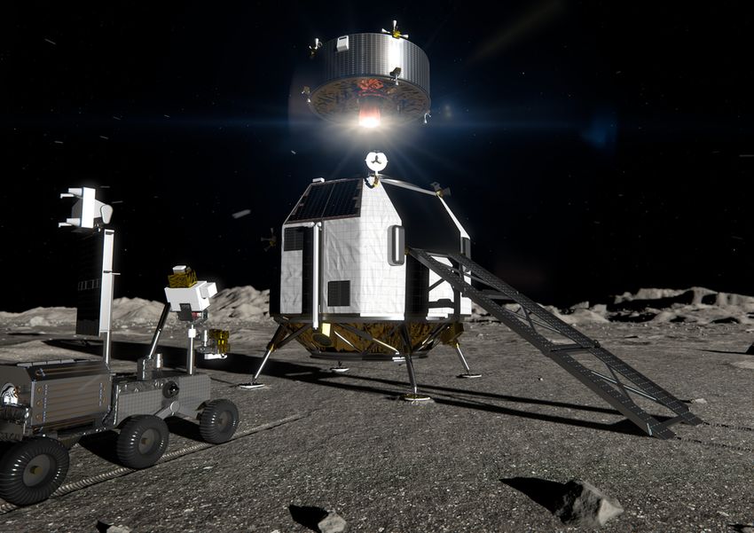
representation of the lunar ascent vehicle, which would rendezvous with a station in orbit.
Figure 1. Lunar lander structure.
Aerospace 2021, 8, 68                                                                                             3 of 38

                        Figure 2. Rendezvous and berthing.

                              The Heracles project was initially planned with the objective of delivering Moon
                        samples to Earth on NASA’s Orion spacecraft as early as its fourth or fifth mission. The
                        initial project was set up to be integrated with NASA’s plan to return to the Moon, and
                        to build a permanent station (Gateway) in cislunar orbit. This has now become NASA’s
                        Artemis mission.
                              A small lander with a rover inside weighing around 1800 kg in total would land and be
                        monitored by astronauts from the Gateway. The current status of the mission includes two
                        distinct tasks: the first is to deploy a rover whose objective is the collection of soil samples,
                        the second is to launch a module that will carry samples to the orbiting station. When
                        the ascent module carrying the sample container arrives, the Gateway’s robotic arm will
                        capture it and berth it with the outpost’s airlock for unpacking and transfer of the container
                        to Orion and subsequent unmanned flights to Earth and later on with returning astronauts.
                              The aim of the mission is to prove the advancements in autonomous operations in
                        space, in particular the focus of this paper is on the sequence of phasing and rendezvous
                        of the LAE with the orbiting LOP-G. The first part of the mission starts with the phasing
                        maneuver that sees the transferring of the LAE-also called chaser in the following—with
                        the payload of lunar soil, collected from the south pole of the Moon, from an assumed low
                        lunar orbit with an altitude of 100 km towards the L2 Near Rectilinear Halo Orbit (NRHO)
                        in which the LOP-G—also called target—is orbiting. The rendezvous maneuver will take
                        care of the approach when the relative distance between the two space vehicles is less than
                        100 km.
                              The literature and the technical details will be discussed in the dedicated sections, and
                        the goal of this section is instead to provide a general background for of the challenges that
                        the design of a transfer maneuver in such peculiar environment implies.
                              One of the critical aspects of this problem is the formulation of the proper equa-
                        tions of motion that should be written in non-inertial reference frame and must describe
                        the complete 6-DOF relative dynamics for the rendezvous and berthing; however, un-
                        der the restricted three-body problem hypothesis, there is no closed form solution and
                        no standard procedure to compute the best rendezvous strategy and to select the best
                        guidance/control technique.
                              Phasing maneuvers are continuously performed in low Earth orbit to connect to the
                        ISS, but no experience is available in the case of automated motion in the restricted three-
                        body problem. The LAE must fly towards the Gateway departing from a Low Lunar Orbit
                        to a L2-NRHO, minimizing the fuel consumption and the required time of flight. The
                        degrees of freedom of the maneuver are multiple. A possibility is to take advantage of the
                        manifold theory, with the dynamics being modeled under the circular restricted three-body
                        problem, in order to have a preliminary evaluation of the influence of design parameters
                        such as TOF, number of impulses, and their amplitude.
                              Once the phasing is accomplished, the rendezvous phase may start immediately or
                        after one orbit or two orbits depending on the acquired relative initial conditions. The
                        rendezvous is a critical phase of the approaching strategy, since the two vehicles are very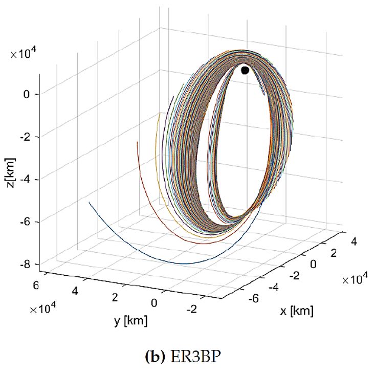
Aerospace 2021, 8, 68 4 of 38
close to one another and the risk of collision or mission abortion is critically high. The
standard closing maneuver usually follows a series of way points located in which the
chaser must stop and check its state and the relative state according to accuracy, changes to
sensor suite, and safety. During the rendezvous, multiple changes of the types of sensors,
guidance, and control methods may be needed; therefore, all of this instrumentation must
be properly selected, modeled, and validated via simulation. One of the main requirements,
for instance, is the use of cameras for information on translational as well as attitude
state variables.
As an example, Figure 3 shows a conceptual scheme of the sequence of the complete
maneuver for the mission under study in the paper.
KOZ
Phasing Rendezvous
Figure 3. Phasing and rendezvous maneuver example.
3. Relative Dynamics Equations of Motion
This section reviews the relative motion of the two spacecraft within the Earth–Moon
system, or, more generally, the motion of three bodies under mutual gravitational attraction.
The design of the rendezvous and docking maneuvers requires an accurate formulation
of the relative motion; in this work, some working hypotheses are made, such as the
elliptic and circular restricted three-body problem hypotheses. In addition, the equations
of motions are formulated in non-inertial frames to make them more useful in the analysis
and synthesis of the GNC loop. The complexity of this formulation stays in the fact that no
closed solution exists for the problem. The interested reader can refer to [2] for more details.
The appropriate reference frames are reviewed herein; then, translational and rotational
dynamics are described.
3.1. Reference Frames
The generic inertial frame centered in O and with unit vectors Î, Ĵ, and K̂, will be
denoted as follows:
I : C; Î, Ĵ, K̂ (1)
Consider two primary bodies, with masses M1 and M2 , orbiting around their compos-
ite center of mass C in a collinear formation. A convenient frame for describing the motion
of spacecraft in such a system is the synodic reference frame. It can be centered in one of the
primaries center of mass, as in [3], and the unit vectors are defined as follows:
• ı̂s = −r12 /kr12 k where r12 is the position of M2 with respect to M1 ;
• k̂s is perpendicular to the plane where the primaries revolve, and is positive in the
direction of the system angular velocity vector;
• ̂s = k̂s × ı̂s completes the right-handed coordinate systems.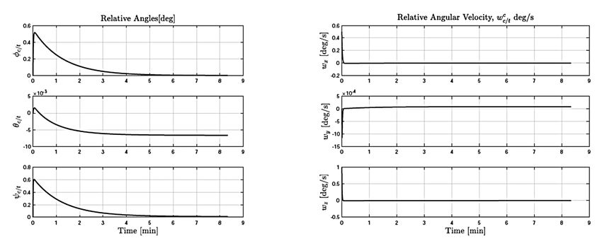
Aerospace 2021, 8, 68 5 of 38
This choice may be convenient when spacecraft measurements are taken with respect
to the nearest primary. For instance, in [3], the Sun–Earth/Moon system is considered, and
the synodic frame is centered on the Earth, since the spacecraft receives measurements with
respect to it. In the following, we will refer to such a coordinate system as primary-centered
rotating frame, and it will be denoted as
n o
Mi : Oi ; ı̂m , ̂m , k̂m (2)
where i is the index of the primary chosen for placing the coordinate frame. Figure 4 shows
the primary-centered rotating frame, centered on M2 , and the Local-Vertical Local Horizon
Frame, described next.
(a) Local-vertical local horizon frame L2 : in the picture, it is
possible to see a schematic representation of the LVLH frame
(b) Primary-centered rotating reference frame M2
Figure 4. Reference frames.
Rendezvous trajectories are generally described in a frame local to the target. This
eases the analysis and the trajectory monitoring of incoming vehicles, as well as the
definition of keep-out zones and admissible approaching corridors. The LVLH frame is
usually employed for rendezvous scenario analysis, and defined as:
n o
Li : rit ; ı̂, ̂, k̂ (3)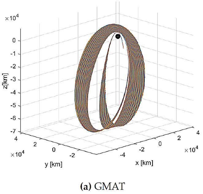
Aerospace 2021, 8, 68 6 of 38
The LVLH (Sometimes called orbital frame) frame is defined with respect to the
primary body around which the target is orbiting. Denoting with rit the target position
with respect to the primary i, with ṙit M , the target velocity as seen from the primary,
i
and with hit = rit × ṙit M , the target specific angular momentum with respect to the
i
primary, the LVLH frame unit vectors are defined and named as follows:
• k̂ = −rit /krit k points to the primary and is called R-bar;
• ̂ = −hit /khit k is perpendicular to the target instantaneous orbital plane (negative
specific angular momentum direction) and is called H-bar;
• ı̂ = ̂ × k̂ completes the right-handed reference frame, and is called V-bar.
The above definition of the LVLH frame is consistent with the one given by Fehse in its
classical reference book for spacecraft rendezvous and docking [4] (pp. 31–32, Section 3.1.3).
The LVLH frame for a target orbiting around M2 is shown in Figure 4.
Note that the formal definition of the LVLH frame is relative to Kaplerian motion so
using R-bar, H-bar, and V-bar is somewhat an abuse of notation, justified by their use in
the community. In addition to the above, other body fixed reference frames can be used to
highlight the dynamics relative to specific points of the vehicles (docking port, geometric
center of mass, location of actuators, etc.).
3.2. Translational Equations of Relative Motion
Consider a target and a chaser spacecraft, orbiting around the Moon, and subjected to
both Earth and Moon gravitational influence. Their equations of motion with respect to the
Moon are:
r r + rem rem
r̈ I = −µ 3 − (1 − µ) − 3 (4)
r kr + rem k3 rem
rc rc + rem rem
r̈c I = −µ 3 − (1 − µ) 3
− 3 (5)
rc krc + rem k rem
where:
• µ = 1.215 × 10⁻² is the Moon–Earth mass ratio parameter defined as:
µ Me − 1
µ = µe +mµm = (1 + M m
) with Me + Mm = 1
• rem is the position of the Moon with respect to the Earth, and rem = krem k its norm;
• r and rc are the target and chaser positions with respect to the Moon, with norms
r = kr k, and rc = krc k, respectively.
In order to simplify computation, distances are normalized to the Moon semi-major
axis and time to the Moon mean angular motion.
With reference to Figure 5, the chaser position with respect to the Moon is given by:
rc = r + ρ (6)
where ρ is the relative position of the chaser with respect to the target. Taking the second
time derivative of Equation (6) and using Equations (4) and (5), we obtain the nonlinear
equations of relative motion in the LVLH reference frame:
ρ̈ L + 2ωl/i × ρ̇ L + ω̇l/i L × ρ + ωl/i × (ωl/i × ρ)
r r+ρ r + rem r + ρ + rem
=µ 3− + (1 − µ ) − (7)
r kr + ρ k3 kr + rem k3 kr + ρ + rem k3
Recall that:
ω̇l/i I
= ω̇l/i L (8)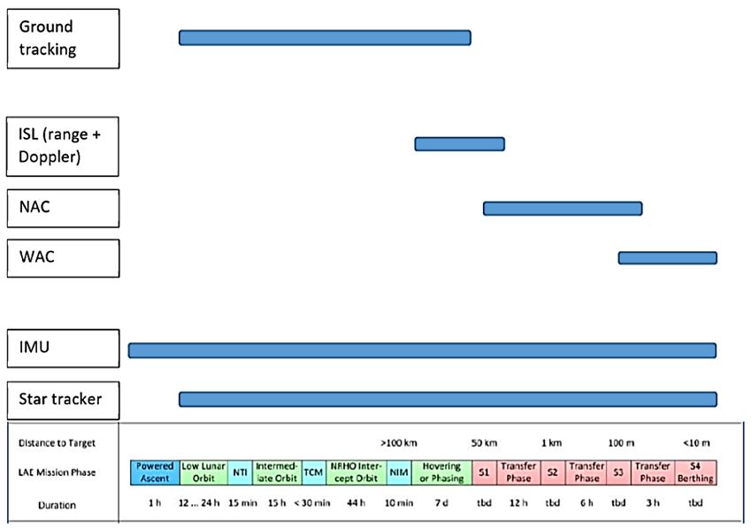
Aerospace 2021, 8, 68                                                                                            7 of 38

                        Figure 5. Target and chaser spacecraft in the three-body system.

                             Using the subscript notation for the reference frames above, the angular velocity of
                        the LVLH frame with respect to the inertial frame can be computed by simple composition:

                                                              ωl/i = ωl/m + ωm/i                                    (9)

                        where ωl/m and ωm/i are the angular velocities of L with respect to M, and of M with
                        respect to I , respectively. The LVLH angular acceleration with respect to I is given by:

                                   ω̇l/i L = ω̇l/m L + ω̇m/i L = ω̇l/m L + ω̇m/i M − ωl/m × ωm/i               (10)

                            Equation (7), along with Equations (9) and (10), constitutes a set of time-varying
                        nonlinear equations:

                        •    r, ωl/m , and ω̇l/m L that depend on the target motion around the Moon;

                        •    rem , ωm/i , and ω̇m/i M , characteristics of the Moon orbital motion.
                              Equation (7) can be further simplified if we consider the restricted three-body problem
                        (elliptic or circular), which will be actually used later on in the paper for the guidance
                        design.

                        3.3. Attitude Equations of Motion
                              Traditionally, orbital mechanics refers to trajectory dynamics; however, in our problem,
                        attitude motion becomes especially critical in order to maintain correct orientation in the
                        final phase (berthing or docking).
                              Standard derivation using rigid body approximation uses Euler’s rotation equations
                        with the general form [5]:

                                                               Iω̇ + ω × Iω = N                                   (11)
                        where N is the vector of external torques, I is the inertia tensor matrix, and ω is the angular
                        velocity about (typically) the principal axes.
                             As angular velocity vectors are cumulative, we can write the inertial angular veloc-
                        ity as:
                                                               ω = ωco + ωoi
                        where ω is the angular rate of body chaser frame w.r.t. inertial frame, ωco (or ωc ) is the
                        angular rate of body chaser frame w.r.t. orbital frame and ωoi is the angular velocity of
                        orbital frame w.r.t. inertial frame. Note that all vectors are expressed in chaser body frame.
                        For the kinematics, we derive the differential equations of motion of the body frame w.r.t.
                        the LVLH reference frame, relating the Euler angles (in their Bryant 3, 2, 1 sequence) with
                        the angular velocity vector ωc [6,7]. Using the standard Euler matrix rotation, we can write
                        ωc as a function of Euler angles. The inverse relationship becomes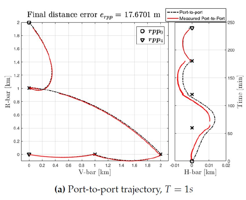
Aerospace 2021, 8, 68 8 of 38
θ̇ x cos(θy ) sin(θ x ) sin(θy ) cos(θ x ) sin(θy )
1
θ̇y = 0 cos(θ x ) cos(θy ) − sin(θ x ) cos(θy )ωc = J(θc )−1 ωc (12)
cos(θy )
θ̇z 0 sin(θ x ) cos(θ x )
Quaternions can also be used if singularities are critical. The interested reader can
refer to [5,6], for instance.
The target’s attitude model is taken from the literature to be a saw tooth type of
motion, with an amplitude of one degree and a frequency of 1 Hz [4,7].
3.4. Attitude Relative Motion
The relative attitude between the two spacecraft is based on the angular rate vectors,
since Euler angles are not cumulative. Thus:
ωra = ωc − Rco (θc )ωt (13)
where ωra is the relative angular rate in chaser body frame, ωc is the chaser angular rate
expressed in chaser frame, ωt is the target angular rate expressed in orbital frame and
Rco is the rotation matrix that transforms a vector from orbital frame components to body
chaser frame components
− sin(θcy )
1 0 0 cos(θcy ) 0 cos(θcz ) sin(θcz ) 0
Rco (θc ) = 0 cos(θcx ) sin(θcx ) 0 1 0 − sin(θcz ) cos(θcz ) 0 (14)
0 − sin(θcx ) cos(θcx ) sin(θcy ) 0 cos(θcy ) 0 0 1
Using Equation (13), we can express the derivative of the relative Euler angles θ̇ra
as follows:
θ̇ra = J(θra )−1 ωc − J(θra )−1 Rco (θc )ωt (15)
where J(θra ) is the appropriate Jacobian matrix.
For close proximity maneuvers, we need the relative centers of mass position of
interest, and the position and velocity between two docking ports, which are located
elsewhere on the spacecraft. The port to port distance can be expressed as
ρ pp = ρ + rdc − rdt (16)
where ρ is the relative distance between chaser and target CoM, rdc and rdt are the docking
port position of chaser and target, respectively. The equation above can be seen as an
output of the system.
The target (or chaser) docking port in the orbital reference frame LVLH can be pre-
sented as
r pi o = Rio (θi ) T r pi i
(17)
with the rotation matrix defined as follows:
cos(θiy ) 0 − sin(θiy )
1 0 0 cos(θiz ) sin(θiz ) 0
Rio (θi ) = 0 cos(θix ) sin(θix ) 0 1 0 − sin(θiz ) cos(θiz ) 0 (18)
0 − sin(θix ) cos(θix ) sin(θiy ) 0 cos(θiy ) 0 0 1
The subscript i = c, t indicate chaser or target, respectively.
4. Validation of the Equations of Motion
This section describes in detail the validation process performed by comparing the
model of the previous section with available Ephemeris models. The dynamics of the target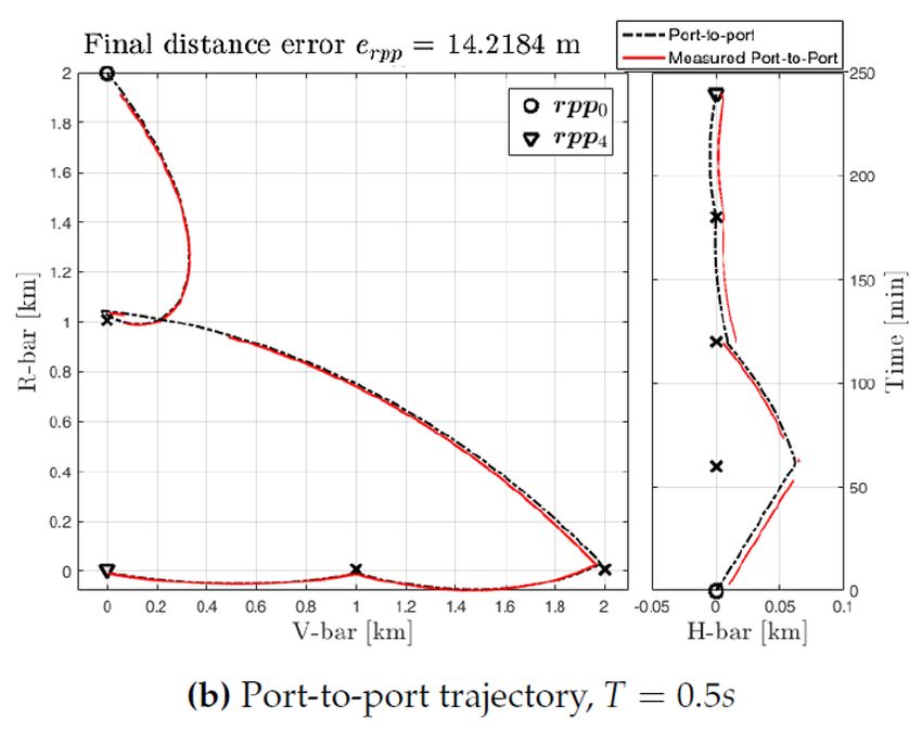
Aerospace 2021, 8, 68                                                                                           9 of 38

                        orbit, relative ER3BP, and CR3BP motions are evaluated for a free drift motion and the
                        most significant rendezvous scenario.
                             The Ephemeris model was not directly implemented and the validated commercial
                        software GMAT was selected [8], since it could be easily integrated with the propagation
                        simulator. The set DE405 generated by JPL was used in the comparison.

                        4.1. Propagation of the Equations of Motion
                             This section presents the propagation of equations of motion over one target orbit
                        with no active corrections. The comparison was performed in the following way:
                        Elliptic restricted, circular restricted, and GMAT were initialized with the same initial
                        conditions in terms of position and velocity in the synodic reference frame S , and the
                        dynamics were propagated for one orbit. The same procedure was performed for 100 times
                        at different Mean Anomalies (M), from 0 to 180 degrees. The one orbit propagation
                        considered to account for a second rendezvous was necessary if the first was not successful.
                        GMAT was set to simulate the restricted three-body problem dynamics as well.
                             The orbit propagation in the three different models (GMAT, ER3BP, CR3BP) is shown
                        in Figure 6; in each sub figure, it is possible to see all the trajectories propagated for the
                        duration of seven days. The propagation duration is taken as representative of the orbital
                        period of the target vehicle; even though the Ephemeris propagation is more realistic, the
                        obtained trajectories require some active corrections to be considered orbits. The starting
                        point at the periselene propagation is in blue, whereas, at the aposelene, it is in red.

                        Figure 6. Propagated trajectories.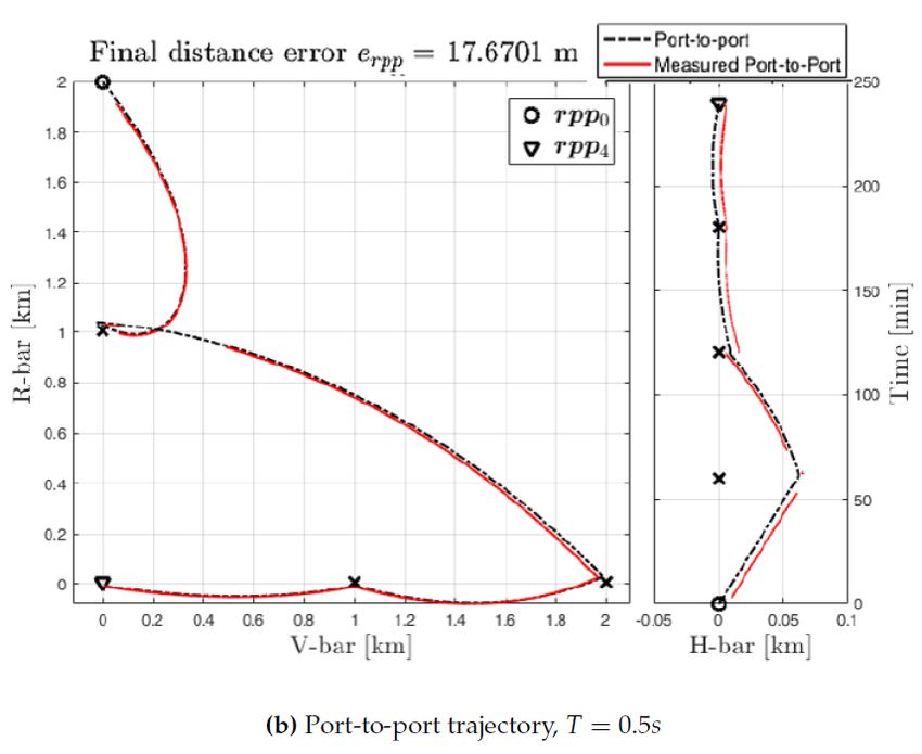
Aerospace 2021, 8, 68                                                                                                    10 of 38

                                   4.1.1. Comparison Results
                                         The next figures and present the comparison between ER3BP, CR3BP, and GMAT.
                                   Figure 7 shows the position (top column) and velocity (bottom column) differences between
                                   ER3BP and GMAT for one orbit period and the details at the aposelene. The numerical
                                   maximum and minimum values are reported in Tables 1 and 2. Note that the aposelene
                                   region is the one that is assumed to provide better rendezvous properties. The position
                                   error increases with the simulation time, and it increases more rapidly as the starting point
                                   is closer to the periselene. This latter result is expected since the unmodelled dynamics
                                   play a larger role.
                                         Analogous tests were performed using the CR3BP and shown in Figure 8 by using the
                                   same simulation procedure. It is possible to observe that, as expected, the CR3BP model
                                   has larger errors with respect to the Ephemeris than the ER3BP model. Moreover, the
                                   error amplitude can be tolerated for mean anomalies between 100 and 180 degrees. The
                                   numerical errors in Tables 1 and 2 indicate the values propagated trajectory with respect
                                   to GMAT. The tables highlight how the propagation errors increase with the three-body
                                   restricted models with respect to the Ephemerides.

                        (a) Position comparison                                (b) Position comparison-aposelene

                        (c) Velocity comparison                                (d) Velocity comparison-aposelene

                                             Figure 7. ER3BP and Ephemeris comparison.

                                   Table 1. Maximum propagation errors.

                                                                              ER3BP                         CR3BP
                                            Position Error                 7.2 ×10⁴  km                  7.35 × 10⁴ km
                                            Velocity Error                   1.8 km/s                       1.8 km/s
                                      Position Error-Aposelene                 800 km                        556 km
                                      Velocity Error-Aposelene               0.01 km/s                    0.009 km/s
Aerospace 2021, 8, 68 11 of 38
Table 2. Minimum propagation errors.
ER3BP CR3BP
Position Error 2.3 ×10⁴ km 1.755 × 10⁴ km
Velocity Error 0.006 km/s 0.003 km/s
Position Error-Aposelene 255 km 424 km
Velocity Error-Aposelene 0.003 km/s 0.005 km/s
(a) Position comparison (b) Position comparison-aposelene
(c) Velocity comparison (d) Velocity comparison at Aposelene
Figure 8. CR3BP and Ephemeris comparison.
4.1.2. Solar Radiation Pressure (SRP)
Since the presence of the solar radiation pressure SRP was initially neglected in the
derivation of the equations of motion, a preliminary evaluation of its influence was also
assessed on the dynamics of the single spacecraft and on the relative dynamics. The solar
radiation pressure is generated by electromagnetic waves that imprint a pressure on the
surfaces hit by the waves themselves. There are many models depending on the spacecraft
geometry and orbital properties; see [9], for instance. Here, the pressure is modeled as
in [10] and given by:
Φ
P= E (19)
c
where Φ E is the energy flux associated with the electromagnetic wave spectrum, and
c = 299,792,458 m/s is the speed of light. The pressure acts on every exposed surface,
and it can influence the motion of the chaser and target vehicles. For additional details,
see [10]. In GMAT, the solar radiation pressure model is considered as a spherical radiation
from the Sun, with a flux of 1376 W/m2 . The tests were performed in GMAT with the
same Ephemeris model used above, and adding the solar radiation pressure assuming an
effective area of 10 m2 for the target and 3 m2 for the chaser. In the first test, the target
free dynamics are propagated and compared with the same dynamics propagated underAerospace 2021, 8, 68 12 of 38
the ER3BP; the second test consists of the relative dynamics between chaser and target
comparison with the the corresponding dynamics under the ER3BP.
The results are summarized in the figures below. Figure 9 shows the propagation
of the target orbit with the influence of the solar pressure compared with the dynamics
propagated under the ER3BP. The difference between the two models differs from the
ones reported in Figure 7 for the shape but not for the order of magnitude. Therefore, the
contribution due to SRP can be considered negligible.
Figure 10 describes the worst case scenario with the orbits propagated in GMAT with
and without solar pressure and the same orbit propagated in ER3BP. Figure 11 shows the
orbits propagated from the aposelene.
The free motion of the relative dynamics is also compared with the ER3BP with and
without the presence of the SRP; see Figures 12 and 13. In the latter, the propagation
is performed for one entire orbit, and, as expected, the maximum amount of error is
accumulated at the passage at the periselene; after that, the errors decrease again.
(a) Free dynamics comparison with solar radiation pressure
(b) Free dynamics comparison with solar radiation pressure,
Aposelene
(c) Free dynamics comparison with solar radiation pressure,
Velocity
Figure 9. ER3BP and Ephemeris comparison—Solar radiation pressure.Aerospace 2021, 8, 68 13 of 38
Figure 10. Worst case scenario orbit comparison.
Figure 11. Orbit comparison-Aposelene.
(a) Relative Dynamics comparison, Position (b) Relative dynamics comparison, Velocity
(c) Relative Dynamics comparison SRP, Position (d) Relative Dynamics Comparison SRP, Velocity
Figure 12. Relative dynamics ER3BP- Ephemeris comparison with and without SRP.Aerospace 2021, 8, 68 14 of 38
(a) Relative Dynamics comparison, Position (b) Relative dynamics comparison, Velocity
(c) Relative Dynamics comparison SRP, Position (d) Relative Dynamics Comparison SRP, Velocity
Figure 13. Relative dynamics ER3BP- Ephemeris comparison with and without SRP.
The presence of the SRP changes the shape of the error of the relative dynamics a
bit, but the amplitude of the errors stays in the same order of magnitude. The maximum
amount of position error is obtained when the dynamics are propagated starting from the
periselene; the maximum amount of velocity error is obtained when the two vehicles pass
through the periselene, as expected.
The maximum and minimum relative motion errors with and without SRP are shown
in Tables 3 and 4, respectively. The relative errors remain very limited and the maximum
position value must be taken into account when designing a trajectory that is safe with
respect to imposed keep-out-zones.
Table 3. Maximum relative dynamics errors.
NO-SRP SRP
Position Error 44.95 km 46.57 km
Velocity Error 17.61 m/s 18.02 m/s
Table 4. Minimum relative dynamics errors.
NO-SRP SRP
Position Error (1 Orbit) 8.3 km 9.09 km
Velocity Error (1 Orbit) 6.2 × 10⁻⁵ km/s 5.3 × 10⁻⁵ km/sAerospace 2021, 8, 68 15 of 38
5. Sensors and Actuators’ Models
One of the important elements introduced in the equations of motion is a character-
ization of sensors and actuators. The selection is based on the assumed choice for the
rendezvous mission and improves the accuracy of overall dynamic behavior. The following
sections provide a general description of component suites, their models, and validity. We
remind the reader that the motivation for component selection is based on the relative
effectiveness for the mission at hand, rather than a theoretical optimization evaluation. In
particular, cameras are selected to play a primary role in the relative position measurement.
5.1. Sensors
Due to the characteristics of the mission, the set of sensors used by the guidance and
control depends on the relative distance between chaser and target, which selects which
suite is active at any particular moment. A qualitative representation is shown in Figure 14.
Figure 14. Chaser navigation concept.
Of particular interest are:
• Inter Satellite Link
• Wide Angle Camera
• Narrow Angle Camera
ISL, WAC, and NAC were implemented in the model as a single block, with the active
sensor selected in relation to the relative distance between chaser and target, with the
amount of error committed by the selected sensor’s suite used to define the working ranges
of each set-up. The main camera parameters are shown in Figure 15.Aerospace 2021, 8, 68 16 of 38
Zc
Xc
α
αc
Camera Yc β α1
R
l h
Target
Figure 15. Reference quantities and Camera frame.
Range estimation using the NAC is computed according to:
ang px
RangeError% = 0.5 100 (20)
2α1
The error is a function of the relative distance R as shown in Figure 16.
Figure 16. Percentage of range error estimate with NAC.
If the distance is above 10 km, the sensor used to estimate the range is the ISL; in fact, it
commits an error in the range estimation equal to 3%R, and, looking at Figure 16, it is possible
to notice that the range estimation error produced by the NAC is above 3% for ranges larger
than 6 km. The NAC is also used for the measurement of the lateral displacement (α and β)
and an error of 100% of the target angular visible size is taken into account (about 1–2 px)
at large distances.Aerospace 2021, 8, 68 17 of 38
At medium distances (10 km–1 km), the ISL is deactivated and the range is estimated
using the NAC using Equation (21):
ang px
l cos αc
Rerr = + sin αc ± 0.5 (21)
2 tan α1 2α1
where:
• l is the target length that is equal to 5 m;
• αc is the measured azimuth angle of the target center of mass, affected by an error of
100% of the target illuminated size.
• α1 is the difference between the azimuth of the centre of the illuminated zone and the
azimuth of a side of the illuminated zone.
• ang px the pixel angular size of the visible Target area.
The lateral displacement is still measured with the NAC and the relative is between 5
and 100 px (100% of the target illuminated side). The lateral displacement error is computed
using Equation (22), and the trend is reported in Figure 17.
The angular error αerr defines the limits between medium distances and short dis-
tances; in fact, medium distances are considered those for which RangeError% is less than
3%R, but the lateral displacement error, computed with Equation (22), is less than 100 px;
as a result, the medium distances are those included in the range 1–10 km:
l
αerr = arctan (22)
R
1000
900
800
700
600
500
400
300
200
100
0
0 1 2 3 4 5 6 7 8 9 10
Figure 17. Lateral displacement error.
The short distances are considered those between 1 km and 5 m; here, the sensor used
is the WAC and the error on lateral displacement is equal to 0.2%R and the error on R is
2%R. At short distances, it is also possible to estimate the relative attitude, with an error of
5 degrees maximum.
The estimation of the translational velocity is based on the differentiation principle
and a subsequent Kalman filtering procedure; however, in this work, the entire navigation
chain is modeled as in Equation (23):Aerospace 2021, 8, 68 18 of 38
ρ̇˜ pp = ρ̇ pp + kρ̃ pp − ρ pp knρ̇ pp (23)
where ρ˜˙pp is the relative port-to-port velocity affected by the error, ρ ˙pp is the velocity
without errors, ρ˜pp is the relative position affected by error, ρ pp is the relative position, and
nρ̇ pp is a white noise.
A similar approach was used to model the angular velocity error, as described in
Equation (24)
ω̃ = ω + kθ̃ − θknω (24)
where ω̃ is the relative angular velocity affected by the error, ω is the velocity without
errors, θ̃ is the relative attitude affected by error, θ is the relative attitude, and nω is a white
noise. Both nρ̇ and nω characteristics can be selected by the user.
The performance of the sensors with the estimated range measurement is shown by
the port-to-port trajectory in Figure 18 drawn in red, representative of a V-bar approach to
the target.
Figure 18. Port-to-port maneuver with the measured range.
It is important to remark that the range is measured with the camera only when the the
target is within the camera field of view; the sensors are initialized at every hold-point and
the sensor suite changes only in the hold-points depending on the target-chaser distance at
hold-point. The camera is also used to measure the relative attitude for short distances as
shown in Figure 19. The range measurements are always available since we assume the
implemented controllers capable of keeping the target within the camera’s FOV.Aerospace 2021, 8, 68 19 of 38
Figure 19. Relative angles with their measurements.
5.2. Actuators
In general, the set of actuators implements the firing command sequences, and allows
the vehicle to separate the motion along different axes and the translational motion from
the rotational one. With reference to the Heracles mission, the propulsion is implemented
by a main engine and 16 RCS-thrusters of 10N each [11] located on the edges of the chaser
vehicle. In this paper, we limit ourselves to describe the model the latter, synthetically
shown in Figures 20 and 21. The main sources of errors are thrust magnitude errors, thrust
direction errors, rise/fall time, and delays.
Figure 20. 3D CAD rendering of the chaser thruster architecture.
The sixteen engines magnitude can be modeled as:
F̄ = F · η1BIT · (1 + δη1BIT ) (25)Aerospace 2021, 8, 68 20 of 38
where F is the nominal thrust level at steady state condition, η1BIT is the theoretical bit
efficiency, and δη1BIT is the impulse bit efficiency random variation. As said before, in our
scenario, F is equal to 10N.
Figure 21. CAD rendering of the chaser thruster architecture-side view.
The theoretical impulse bit efficiency is computed from the empirical formula given
by Equation (26), which is based on the duration of the thruster firing command ton and
the thruster off-time:
− c1
1000ton +c2 /1000to f f
η1BIT = e (26)
ton and to f f are expressed in seconds, and c1 and c2 are the efficiency factor constants.
According to [12], ton and to f f can be selected using a PWM approach. The random
variation of the impulse bit efficiency δη1BIT is assumed to be Gaussian with zero mean
and the standard deviation ση1BIT , given by Equation (27).
σηcoe f 2
ση = min(max (σηmin , σηcoe f 1 · (1000ton ) ), σηsat ) (27)
The misalignment is mainly composed of two contributions: internal and external.
The internal error is due to a misalignment between thrust vector and flange. They
are constant over a single thruster firing, but they change randomly from one firing to the
next, so the internal uncertainty is assumed to behave as a Gaussian noise. The external
errors are due to some misalignment between flange and master reference cube.
The uncertainties remain constant for the entire simulation, but they change from a
simulation to the other. As a consequence, the external uncertainty is assumed to behave
as a uniformly distributed variable.
In addition to magnitude and direction uncertainty, it is necessary to also take into
account the Rise/Fall time behavior [7]. The thrust is discretized following a PWM logic.
The motors have a dynamic and minimum ton and to f f times. The Rise/fall times are taken
into account through a filtering operation: the PWM signal will be filter by a 1st or 2nd
order filter according to Equations (28) and (29). In the filter equation, we can also take
into account a time delay τ:
A −τ
F1 = e (28)
s+b
ωn2 e−sT∆v
F2 = e−τ (29)
s2 + 2ζωn s + ωn2Aerospace 2021, 8, 68 21 of 38
The location of the thrusters depends on the vehicle, its configuration, geometry,
and mission. Thus, the contribution that each actuator gives to torques and forces can
be computed with respect to the chaser center of mass in the body frame axis, which is
the Geometrical frame, defined earlier. Due to the absence of data, the chaser vehicle is
considered as a perfect cylinder with uniform density and constant mass; therefore, the
body reference system—that coincides with G in this case—was located along principal
axes of inertia.
The relationship between the thrust of each motor and the torques and forces produced
is then computed by projection. Let us define: Fs , the vector that contains all the thrust
provided by the small thrusters:
T
Fs = F1 F2 ... F16 (30)
The 6x1 vector of forces and torques, in chaser body frame, is called τ, and it is
defined as:
T
τ = Fx Fy Fz Nx Ny Nx (31)
The relation between τ, Fs and Fb is a linear relationship given by Equation (32):
τ = [ Bs ] Fs (32)
where Bs is called the 6 × 16 control allocation matrix [5].
Control allocation is an area with a large amount of literature and many algorithmic
techniques, spanning from structural geometry approaches, to several types of optimization
methods. Ref. [13] is especially interesting for our application; in fact, it avoids the use of a
PWM module after the control allocation because it computes the optimal combination of
duty-cycle to minimize a linear cost function given by:
J = f T [δ1 , . . . , δn ], f = [1 1 . . . 1] T (33)
where [δ1 , . . . , δn ] is the vector that contains the duty-cycles; each element of this vector is
included between 0 and 1, and Fs = Fm ax [δ1 , . . . , δn ], where Fm ax is the maximum thrust
supplied by a thruster. It defines the control law in (32).
Another advantage of this technique is that, by minimizing the duty-cycle vector, the
fuel-consumption is minimized as well because it is proportional to the summation of all
thruster on time. For the reasons briefly explained above, also supported by empirical
results, one of the selected control allocation techniques for comparison is the one proposed
by [13]. Clearly, the selection of a specific allocation algorithm also depends on safety
factors and software computational power specific for space applications. Therefore, a
look-up table approach was also investigated in this study.
The control allocation methods described above are described in detail in Refs. [13,14],
and the interested reader is referred to them. In the following, we only present rendezvous
simulation results as a function of PWM working frequency (1 Hz and 2 Hz, respectively).
The optimal control allocation in Equation (33) selects an optimal combination of Pulse
Width Modulation duty cycle at each step—in the sense that it minimizes the summation
over all duty-cycles and, consequently, the fuel consumption. The optimization method is
the interior-point-legacy (default) and the optimization procedure was executed at each
step using available routines. The rendezvous maneuver simulation is shown in Figure 22,
indicating better performance with a higher PWM frequency.Aerospace 2021, 8, 68 22 of 38
Figure 22. Trajectories varying the PWM frequency (optimal allocation).
In the look-up table algorithm, the thruster modulator is the on-board function that
computes parameters for the actuation of the thrusters during a control cycle. The main
objective is to compute the percentage of the total duration of the control cycle for which
each thruster must be open such that that the average effect of the thrusters over the control
cycle results in a force and torque as requested by the controller. The resulting trajectories
are shown in Figure 23, for the same frequency range.Aerospace 2021, 8, 68 23 of 38
Figure 23. Trajectories varying the PWM frequency (Look-Up table).
Using the Heracles mission data, a comparison in terms of thrust consumption is
shown in Table 5. The table displays the integral of the acceleration at the thruster during
the entire maneuver duration. The “ideal” implies a simulation performed using perfect
sensors and actuators, while “non-ideal” indicates results obtained with more accurate
models for sensors and actuators as described earlier.Aerospace 2021, 8, 68 24 of 38
Table 5. Thrust comparison.
Thrust Consumption
Optimal allocation ideal 15.4 m/s
Optimal allocation non-ideal 16.1 m/s
LUT ideal 22.1 m/s
LUT non-ideal 27.1m/s
6. Rendezvous Guidance and Control
A rendezvous guidance profile is generally composed of several elements aimed
at steering the chaser towards the target, moving between a set of control points. In the
Keplerian case, these trajectories are the result of the application of impulsive or continuous
thrust firings along prescribed directions. Except for very small relative distances, the
maneuvers are computed in an open-loop fashion, and can be based on the solution of the
Hill’s equations [4], for instance. The accuracy of the Hill’s equations for the restricted-
three-body problem is poor and may compromise the good execution of the maneuver,
especially due to their open-loop implementation; therefore, in this section, some of the
maneuvers used for rendezvous and docking are reproduced exploiting the linearized
elliptic ELERM and circular CLERM equations, whose derivation can be found in [2],
together with their range of validity along the target orbit.
The linearization procedure yields a linear time varying expression in state variable
form given by:
ẋ = A(t) x + Bu (34)
with A ∈ R6×6 defined as:
03×3 I3
A(t) = (35)
Aρ̇ρ (t) −2Ωl/i (t)
rr T 1−µ (r + rem )(r + rem )T
µ
Ω̇l/i L − Ω2l/i
Aρ̇ρ = − − 3 I−3 2 − I−3 (36)
r r kr + rem k3 kr + rem k2
with state variable defined in Equation (7). The difference between ELERM and CLERM in
Equation (34) is due to the angular velocities assumption between elliptic and
circular motions.
The closed-form solution of the these equation sets is not straightforward, due to the
presence of time-varying parameters, and the absence of general analytical solutions for
ER3BP and CR3BP orbits. To deal with this problem, different guidance approaches are
introduced. The selection of the guidance algorithm is influenced by the relative distance,
the required level of accuracy, the capability of closing the loop, and the available/current
sensor’s and actuator’s suite. We must remark that the aim of the paper is not to propose
the best guidance algorithm, rather to provide a suitable choice for the mission. Figure 24
shows a sequence of algorithms that are used in the paper. The mathematical details are
reported in the Appendix A. The methods used for the guidance are:
• Adjoint Guidance.
• PID.
• SDRE.
The first two techniques are used to control the relative translational motion and
the absolute attitude motion outside of a safety area defined to avoid collision, and they
operate in an open loop fashion for large to medium distances. The third controller takes
care of the regulation of the attitude and the position in the last part of the approach.Aerospace 2021, 8, 68 25 of 38
Figure 24. Schematic explanation of the guidance sequence.
6.1. Adjoint Guidance
Adjoint models (or more properly dual models) have been extensively exploited for the
solution of classical missile guidance problems, see [15,16], and more recently in [17,18].
They appear to be well suited due to the time varying nature of the relative dynamics. The
application of adjoint theory to our problem is described in Appendix A.1.
The main idea is to consider the relative dynamics as described by ELERM (or in a
simpler model CLERM) as given by Equation (A1), with time response at some finite time
t f > t0 given by Equation (A3). We can associate with Equation (A1) a dual system at time
t f [19] given by Equation (A4), whose initial time response coincides with the final time
response of the original system.
The adjoint guidance is applied in this work to a two-impulse maneuver at each hold
point. In other words, the chaser leaves a hold point with an impulsive firing and reaches
the next with a braking impulse. The total input has the form given by Equation (A8)
with two impulses applied at times t1 and t2 ; then, we obtain relative position and rate
from Equation (A15), where (ρ f , ρ̇ f ) is the desired relative state, computed starting from
ELERM.
The performance of the guidance was evaluated computing relative distance and
velocity errors repeated here for clarity’s sake:
eρ = kρ f − ρ(t f )k, eρ̇ = kρ̇ f − ρ̇(t f )k (37)
with total control effort: Z t
f
∆V = ku(t)kdt (38)
t0
6.2. PID Guidance Controller
During the initial phase of the rendezvous, the primary concern is to follow a pre-
scribed attitude profile, or to maintain the target in the field of view of the chaser’s cameras.
To this end, a standard PID controller on all axes was considered to be satisfactory. The
controllers were simply tuned to obtain a good rise time.
An example of the performance without and with the controller is shown in
Figure A1 and Figure A2, respectively. The simulation considers a nonzero initial condition
on the angular velocity with no damping at the beginning of the maneuver. The continuous
rotation of the vehicle can be seen in Figure A1. After the insertion of the controller, the
vehicle is stabilized to the desired attitude (zero in this case) as shown in Figure A2. The
presence of the PID also allows the pointing of the cameras always towards the targetAerospace 2021, 8, 68 26 of 38
avoiding possible singularity issues (of course, the equations can be always transformed in
their quaternion, not changing the general controller philosophy).
Two different attitude-modes are available for large and medium distances, where
the PID is in charge of controlling the attitude of the chaser. In the former case, the chaser
is forced to follow a user-defined attitude profile w.r.t the LVLH; this profile is defined
in Euler angles. In the latter case, the chaser must point always towards the target to
keep it inside the camera FOV, with the dynamics expressed either in Euler angles or
quaternions [20].
In the latter, the quaternion (qre f ) that represents the angular displacement between
the camera axis and the target position w.r.t. the chaser being computed first. Then, it is
used as a reference for the controller; this means that the controller is asked to zero the
chaser attitude w.r.t qre f . To compute qre f , let us define nre f and θre f as in Equations (39)
and (40):
xc × (−ρ)
nref = (39)
kxc × (−ρ)k
kxc × (−ρ)k
θre f = arctan (40)
xc · (−ρ)
Combining the equations yields:
θre f θre f
qre f = [cos( ); nre f sin( )] (41)
2 2
The quantities written in Equations (39)–(41) are graphically represented in Figure 25.
Chaser Zc
Xc
qref
-ρ
Yc
Target
Figure 25. Target pointing strategy.
At close distances, the user can only define the desired relative attitude profile; in
other words, the user can define the attitude of the chaser w.r.t. the target at each hold-point
that is located at a close distance from the target.
6.3. SDRE Guidance
Since the middle of the 1990s, State-Dependent Riccati Equation (SDRE) strategies
have emerged as a general design structure that provide a systematic and effective means
of designing nonlinear controllers, observers, and filters. These methods overcome many
of the difficulties and shortcomings of existing methodologies, and deliver computationally
simple algorithms that have been highly effective in a variety of practical and meaningful
applications. In a special session at the 17th IFAC Symposium on Automatic Control
in Aerospace 2007, theoreticians and practitioners in this area of research were brought
together to discuss and present SDRE-based design methodologies as well as review
the supporting theory. It became evident that the number of successful simulations,
experimental, and practical real-world applications of SDRE control have outpaced the
available theoretical results.
The methodology originated as an extension of Linear Quadratic Control techniques
to a special class of nonlinear systems. An interesting survey on the method can be found
in [21]. Stability and controllability aspects are discussed in [22,23]. SDRE controllers wereAerospace 2021, 8, 68 27 of 38
used in space related applications, especially for the control of proximity operation and
formation flight as reported in [24–26].
The method entails a factorization (that is, parameterization) of the nonlinear dynam-
ics into a state vector and the product of a matrix-valued function that depends on the
state itself. In doing so, the SDRE algorithm fully captures the nonlinearities of the system,
bringing the nonlinear system to a (non unique) linear structure having state-dependent
coefficient matrices, and minimizing a nonlinear performance index having a quadratic-like
structure. A state dependent algebraic Riccati equation P using the SDC matrices is then
solved online to give the suboptimum control law.
A more detailed derivation can be found in Appendix A.3. The structure of the control
law, in its simpler form that assumes the measurement of the entire state, is a full state
feedback controller given by Equation (A25):
u = − R−1 (x )B> (x )P (x )x
The procedure can be applied in the presence of inequality constraints as well, derived
from a set of admissible states on relative position and velocity, especially at close distances,
where relative motion precision is necessary as shown in Equation (A26). The resulting
control law then becomes:
u = −K(x)x
= − K0 ( x ) + K Ω ( x ) x
Here, the gain matrix includes the constraint term KΩ . A constrained proximity representa-
tion is shown in Figure A3 of Appendix A.3, with the constraints derivation.
A numerical simulation is shown below using the initial conditions in Table 6. We
assume that the attitude motion of the target has a maximum amplitude of 5°. For the
chaser, the inertia matrix is I = 10−3 · diag(1.1, 0.6, 0.6) kg · m2 . The direction vector of
approaching cone is [p]T = [−1, 0, 0]> , and the maximum cone angle is set as β = 25°.
Table 6. Initial attitude condition.
Variable Data
qc/l [1.0, 0, 0, 0.0087]>
ωc/i rad s−1 [0, 0.01, 0]>
qt/l [0.9999, −0.0061, −0.0061, −0.0061]>
ωt/l rad s−1 [0.0019, 0.0019, 0.0019]>
[ρ0 ]L [km] [−10, 0, −4]>
[ρ̇0 ]L km s−1 [0, 0, 0]>
The example was selected to show the performance of the SDRE guidance, assuming
perfect sensor and actuator models. The resulting trajectory is shown in Figure 26.Aerospace 2021, 8, 68 28 of 38
Figure 26. Approaching constraint example.
7. Full Rendezvous Sequence
This section describes an example of full rendezvous/berthing maneuver, using the
methodologies described in the paper.
As shown in Section 4, the simulation uses the Ephemeris model, in particular the
DE430 provided by JPL. The hold-point settings for the maneuver are given by:
• HP0 = [−50; −7.6024; 5.9946] km, TOF 40 h;
• HP1 = [−11.4573; −7.6024; 5.9946], TOF 12 h;
• HP2 = [−0.9003; −1.9097; 0.4777], TOF 8 h;
• HP3 = [−0.1; 0; 0], TOF 6 h;
• HP4 = [0; 0; 0];
The location of the hold-points is passively safe [5], and it was selected minimizing
the energy consumption. The duration of the different transfer times is designed to enter
the safety area at the aposelene; moreover, the location of HP0 within the target orbit
corresponds to a mean anomaly of about 113° that guarantees one of the lowest differences
between the Ephemeris equations and the ER3BP equations (inclusive of sensor and
actuator dynamics).
Figure 27 shows the 3D full rendezvous trajectory, Figure 28 show its the R-bar–V-bar
projection, with the safety zone indicated by the circle satisfied until actual berthing occurs.
Figure 27. Rendezvous trajectory.Aerospace 2021, 8, 68 29 of 38
Figure 28. Rendezvous trajectory-LVLH.
Figure 29 shows the relative velocity components between chaser and target. The
relative attitude is shown in Figure 30. In both cases, the contribution of sensors and
actuators models is shown in red as compared to the ideal case (black line).
Figure 29. Relative rendezvous velocity.Aerospace 2021, 8, 68 30 of 38
Figure 30. Relative attitude.
8. Conclusions
The paper presents a comprehensive preliminary analysis of the dynamics and control
issues arising in a rendezvous mission between an active vehicle departing from lunar orbit
to a target station located in an NRHO L2 orbit. The mission requires a three-body problem
description due to the gravity of both Earth and Moon. The implementation of dynamic
components was based on ESA’s Heracles mission data and preliminary configuration. The
accuracy of the model was improved with the inclusion of sensors and actuators models,
and guidance algorithms were selected in order to verify the reliability of the GNC loop.
The validation was presented using an Ephemeris model. The paper shows that elliptic
restricted three-body dynamics offers a good approximation; in fact, since the rendezvous
will occur at the aposelene, the circular restricted model could be used as a starting point
for the guidance design. If the first rendezvous were aborted, the mall errors in the relative
motion would allow a try after one orbit. The selection of guidance algorithms was driven
by feasibility, and a full mission profile was tested successfully in simulation.
Author Contributions: The authors contributed equally. All authors have read and agreed to the
published version of the manuscript.
Funding: This work was partially supported by the European Space Agency under contract No.
000121575/17/NL/hh. The view expressed herein can in no way be taken to reflect the official
opinion of the European Space Agency.
Institutional Review Board Statement: Not applicable.
Informed Consent Statement: Not applicable.
Data Availability Statement: Not applicable.
Conflicts of Interest: The authors declare no conflict of interest.You can also read