Model-Free Quantum Control with Reinforcement Learning
←
→
Page content transcription
If your browser does not render page correctly, please read the page content below
Model-Free Quantum Control with Reinforcement Learning

                                                             V. V. Sivak,1, ∗ A. Eickbusch,1 H. Liu,1 B. Royer,2 I. Tsioutsios,1 and M. H. Devoret1
                                                                     1
                                                                         Department of Applied Physics, Yale University, New Haven, CT 06520, USA
                                                                           2
                                                                             Department of Physics, Yale University, New Haven, CT 06520, USA
                                                               Model bias is an inherent limitation of the current dominant approach to optimal quantum control,
                                                            which relies on a system simulation for optimization of control policies. To overcome this limitation,
                                                            we propose a circuit-based approach for training a reinforcement learning agent on quantum control
                                                            tasks in a model-free way. Given a continuously parameterized control circuit, the agent learns
                                                            its parameters through trial-and-error interaction with the quantum system, using measurements
                                                            as the only source of information about the quantum state. By focusing on the task of quantum
                                                            state preparation in a harmonic oscillator coupled to an ancilla qubit, we show how to reward
                                                            the learning agent using measurements of experimentally available observables. We demonstrate
                                                            by numerical simulations preparation of arbitrary states using both open- and closed-loop control
arXiv:2104.14539v1 [quant-ph] 29 Apr 2021

                                                            through adaptive quantum feedback. Our work is of immediate relevance to superconducting circuits
                                                            and trapped ions platforms where such training can be implemented real-time in an experiment,
                                                            allowing complete elimination of model bias and the adaptation of quantum control policies to the
                                                            specific system in which they are deployed.

                                                                   I.     Introduction                           In a variety of domains, deep reinforcement learning
                                                                                                                 has recently produced spectacular results, such as beat-
                                               Quantum control theory addresses a problem of op-                 ing world champions in board games [13, 14], reach-
                                            timally implementing a desired quantum operation us-                 ing human-level performance in sophisticated computer
                                            ing external controls. The design of experimental con-               games [15, 16] and controlling robotic locomotion [17, 18].
                                            trol policies is currently dominated by simulation-based             Applying model-free RL to quantum control implies di-
                                            optimal control theory (OCT) methods with favorable                  rect interaction of the learning agent with the controlled
                                            convergence properties thanks to the availability of an-             quantum system, which presents a number of unique
                                            alytic gradients [1–3] or automatic differentiation [4, 5].          challenges because quantum systems have large state
                                            However, it is important to acknowledge that simulation-             spaces that are only partially observable to the agent
                                            based methods can only be as good as the underlying                  through projective measurements. For example, the state
                                            models used in the simulation. Empirically, model bias               of a qubit can be described as a point on a Bloch sphere,
                                            leads to a significant degradation of performance of the             but each individual measurement of a qubit observable
                                            quantum control policies, when optimized in simulation               yields a 1-bit random outcome and collapses the state.
                                            and then tested in experiment. A practical model-free al-            Such stochasticity and minimalistic “quantum observ-
                                            ternative to simulation-based methods in quantum con-                ability” is challenging from the perspective of a learning
                                            trol is thus desirable.                                              agent, since it needs to make decisions based on a very
                                               The idea of using model-free optimization in quantum              limited amount of information about the system’s state.
                                            control can be traced back to the pioneering proposal in             The question arises: can classical RL agents efficiently
                                            1992 of laser pulse shaping for molecular control with a             handle quantum-observable environments?
                                            genetic algorithm [6]. Only in recent years has the con-                We propose a modular circuit-based approach for
                                            trollability of quantum systems and the duty cycle of                training a reinforcement learning agent for continuous
                                            optimization feedback loops reached sufficient levels to             quantum control tasks in a completely model-free way,
                                            allow for the experimental implementation of such ideas.             thereby adapting quantum control policies to the specific
                                            The few existing demonstrations are based on model-                  system in which they are deployed. Given a continuously
                                            free optimization algorithms such as Nelder-Mead sim-                parameterized control circuit, the agent learns its param-
                                            plex search [7, 8], evolutionary strategies [9] and particle         eters through trial-end-error interaction with the con-
                                            swarm optimization [10].                                             trolled quantum system, without any human-provided
                                               At the same time, deep reinforcement learning (RL)                knowledge of the system’s wave-function or model of the
                                            [11, 12] emerged as not only a powerful optimization                 system’s dynamics, unlike in related works [19–37] which
                                            technique but also a tool for discovering adaptive con-              we survey in Section II.
                                            trol policies. In this framework, learning proceeds by                  To illustrate our approach with specific examples, we
                                            trial-and-error, without access to the model generating              focus on the task of quantum state preparation in a
                                            the dynamics and its gradients. Being intrinsically free             harmonic oscillator. Harmonic oscillators are ubiqui-
                                            of model bias, it is an attractive alternative to tradi-             tous physical systems, realized, for instance, as the mo-
                                            tional simulation-based approaches in quantum control.               tional degrees of freedom of trapped ions [38, 39], micro-
                                                                                                                 mechanical membranes [40], and electromagnetic modes
                                                                                                                 in superconducting circuits [41, 42]. They are primitives
                                            ∗   vladimir.sivak@yale.edu                                          for bosonic quantum error correction [43–45] and quan-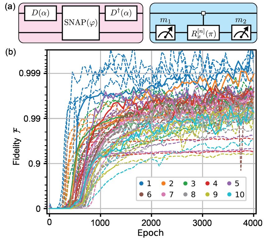
2

tum sensing [46]. Universal quantum control of the os-          III.   Reinforcement learning approach to quantum
cillator is typically realized by coupling it to an ancil-                               control
lary nonlinear system, such as a qubit. In such quantum
environment, ancilla measurements are the agent’s only                       A.   Markov Decision process
source of information about the quantum state in the
vast unobservable Hilbert space and the only source of             We begin by introducing several concepts from the field
rewards guiding the learning algorithm.                         of artificial intelligence (AI). An intelligent agent is any
   For an oscillator-qubit system, we demonstrate how to        device that can be viewed as perceiving its environment
construct task-specific reward circuits by mapping exper-       through sensors and acting upon that environment with
imentally available oscillator observables onto the ancilla     actuators [50]. In reinforcement learning (RL) [11, 12], a
qubit and using qubit measurement outcomes as reward            sub-field of AI, the interaction of the agent with its envi-
bits in the classical training loop. We train the agent         ronment is usually described with a powerful framework
to prepare arbitrary states using both open- and closed-        of Markov decision processes (MDP).
loop quantum control. In the latter case, we leverage the          In this framework, the agent-environment interaction
decision-making power of reinforcement learning to dis-         proceeds in episodes consisting of a sequence of discrete
cover policies for adaptive measurement-based quantum           time-steps. At every time-step t the agent receives an ob-
feedback.                                                       servation ot ∈ O containing some information about the
   Although our demonstration is based on a simulated           current environment state st ∈ S, and acts on the envi-
environment producing mock measurement outcomes,                ronment with an action at ∈ A. This action induces a
the RL agent that we developed (code available at [47])         transition of the environment to a new state st+1 accord-
can be directly applied in real-world experiments.              ing to a Markov transition function T (st+1 |st , at ). The
                                                                agent selects actions according to a policy π(at |ht ), which
                                                                in general can depend on the history ht = o0:t of all past
                                                                observations made in the current episode. In the partially
                    II.   Related work                          observable environment, observations are issued accord-
                                                                ing to an observation function O(ot |st ) and carry only a
   In recent years, multiple theoretical proposals have         limited information about the state. In the special case
emerged around applying reinforcement learning to quan-         of a fully-observable environment, the observation ot ≡ st
tum control problems such as quantum state preparation          is a sufficient statistic of the past and the history carries
[19–27] and feedback stabilization [28], the construction       no more information than the current observation, which
of quantum gates [29–31], design of quantum error cor-          allows to restrict the policy to a mapping from states to
rection protocols [32–35], and control-enhanced quantum         actions π(at |st ). Environments can be further catego-
sensing [36, 37]. However, these proposals are focused          rized as discrete or continuous according to the structure
on recasting the problem in a way that would avoid              of the state space S, and as deterministic or stochastic
facing quantum observability. This is possible only in          according to the structure of the transition function T .
simulated environments, for example by providing the            Likewise, policies can be categorized as discrete or con-
learning agent with full knowledge of the system’s wave-        tinuous according to the structure of the actions space
function, which supplies enough information for decision        A, and as deterministic or stochastic.
making [19, 22–24, 26, 28, 32, 36, 37]. Moreover, since in         The agent is guided through the learning process by a
the simulation the distance to the target state or oper-        reward signal rt ∈ R. The reward is issued to the agent
ation is known at every step of the quantum trajectory,         after each action, but it cannot be used by the agent
it can be used to construct a steady reward signal to           to decide on the next action. Instead, it is used by the
guide the learning algorithm [22–24, 36], thereby allevi-       learning algorithm to improve the policy. The reward sig-
ating the well-known delayed reward assignment prob-            nal is designed by a human supervisor according to the
lem. Taking RL a step closer towards quantum observ-            final goal, and it must indicate how good the new envi-
ability, some works do not give the agent access to the         ronment state is after the agent’s action. Importantly,
wave-function, but still use it for calculation of fidelities   it is possible to specify the reward signal for achieving
and expectation values in different parts of the train-         a final goal without knowing what the optimal actions
ing pipeline [20, 25, 27, 48, 49], which would require a        are, which is a major difference between reinforcement
prohibitive amount of averaging in experiment. Under            learning and more widely appreciated supervised learn-
these various simplifications, there are positive indica-       ing. The goal of the learning algorithm is to find a policy
tions [22, 29] that RL is able to match the performance         π that maximizes the agent’s utility function J, which
of traditional gradient-based OCT methods, albeit in a          in RL is taken to be the expectation J = Eπ [R] of the
simulation where the agent or the learning algorithm has        reward accumulated
                                                                              P          during the episode, also known as
access to extra resources that are not realistically avail-     return R = t rt .
able. Therefore, such RL proposals are not compatible              Even from this brief description it is clear that learn-
with training in experiment, which is required in order         ing environments vary vastly in complexity from “sim-
to eliminate model bias from quantum control.                   ple” discrete fully-observable deterministic environments,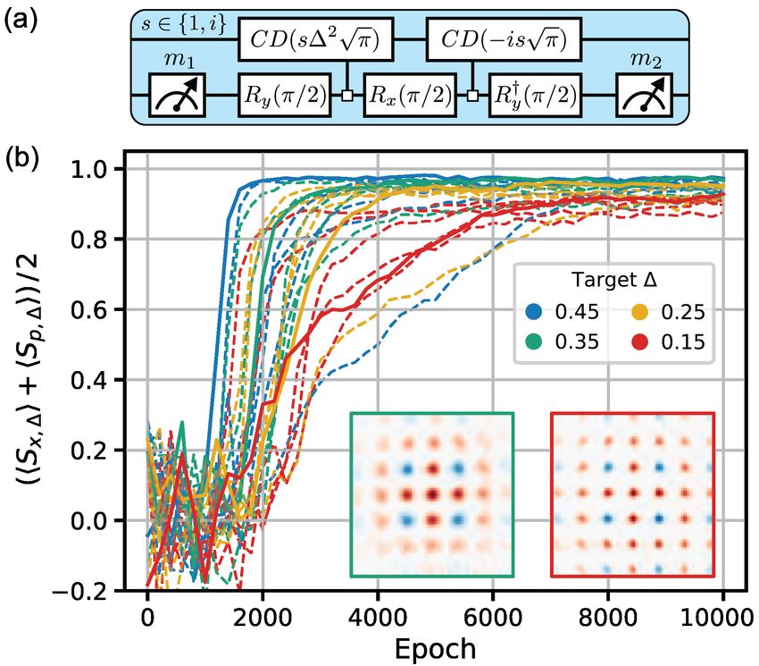
3

                                                                      the two lowest energy levels of a transmon [52]. Note the
                                                                      difference in the use of the term “environment” which in
                                                                      quantum physics refers to dissipative bath surrounding
                                                                      the quantum system, while in our context it refers to the
                                                                      quantum system itself, which is the environment of the
                                                                      agent.
                                                                         It is convenient to abstract away the exact details of the
                                                                      control hardware and adopt the circuit model of quan-
                                                                      tum control. According to such operational definition,
                                                                      the agent interacts with the environment by executing
                                                                      a parametrized control circuit in discrete steps, as illus-
                                                                      trated in Fig. 1. On each step t, the agent receives an ob-
                                                                      servation ot , and produces the action-vector at of param-
                                                                      eters of the control circuit to run in the next time step.
                                                                      The agent-environment interaction proceeds for T steps,
                                                                      comprising an episode. Compared to the typical classi-
                                                                      cal partially-observable MDPs, there are two significant
                                                                      complications in the quantum case: (i) the quantum en-
FIG. 1. The pipeline of classical reinforcement learning ap-          vironment is minimally observable to the agent through
plied to a quantum-observable environment. The agent (yel-            projective ancilla measurements, i.e. the observations ot
low box), whose policy is represented with a neural network,          carry no more than 1 bit of information, and (ii) the ob-
is a program implemented in a classical computer control-
                                                                      servation causes a discontinuous jump in the underlying
ling the quantum system. The quantum environment of the
agent consists of a harmonic oscillator and its ancilla qubit,
                                                                      environment state. While in principle classical partially-
implemented with superconducting circuits and cryogenically           observable MDPs could have such properties, they arise
cooled in the dilution refrigerator. The goal of the agent is to      more naturally in the quantum case. Historically, RL was
prepare the target state |ψtarget i of the oscillator after T time-   benchmarked in richly observable, even if stochastic, en-
steps, starting from initial state |ψ0 i. Importantly, the agent      vironments, and it is therefore an open question whether
does not have access to the quantum-mechanical state of the           existing RL algorithms are well suited for environments
environment, it can only observe the environment through in-          with properties (i)-(ii). There is also a fundamental ques-
termediate projective measurements of the ancilla qubit yield-        tion of whether classical agents can efficiently, in the al-
ing binary outcomes ot . The agent controls the environment           gorithmic complexity sense, learn compressed representa-
by producing at each time-step the action-vector at of pa-            tions of the latent quantum states producing the observa-
rameters of the control circuit (pink box). The reward R for
                                                                      tions, and if such representations are necessary for learn-
the RL training is obtained by executing the reward circuit
(blue box) on the final state |sT i prepared in each episode.         ing quantum control policies. Recognizing some of these
This circuit is designed to probabilistically answer the ques-        difficulties, Ref. [53] introduced “Quantum-Observable
tion “Is the prepared state |sT i equal to |ψtarget i|gi?” A batch    Markov Decision Process” (QOMDP), a term we will
of B episodes is collected per training epoch and used in the         adopt to describe our quantum control framework.
classical optimization loop to update the policy.                        We use the Monte Carlo wave-function method [54] to
                                                                      simulate the quantum environment of the agent. For the
                                                                      environment consisting of an oscillator coupled to ancilla
such as a Rubik’s cube, to “difficult” continuous partially-          qubit and isolated from the dissipative bath, the most
observable stochastic environments, such as those of self-            general QOMDP has the following specifications:
driving cars. Where does quantum control land on this                    1. State space is the joint Hilbert space of the qubit-
spectrum?                                                             oscillator system, which in our simulation corresponds to
                                                                      S = {|si ∈ C2 ⊗ CN , hs|si = 1}, with N = 100 being
                                                                      oscillator Hilbert space truncation in the photon number
              B.   Quantum control as MDP                             basis.
                                                                         2. Observation space O = {−1, +1} is the set of pos-
   To explain how quantum control can be viewed as a                  sible measurement outcomes of the qubit σz operator. If
sequential decision problem, for concreteness we will spe-            the control circuit contains a qubit measurement (closed-
cialize the discussion to a typical circuit QED [42, 51] ex-          loop control), the observation function is given by the
perimental setup, depicted in Fig. 1, although this frame-            Born rule of probabilities. If the control circuit does not
work can be generalized to other physical platforms. The              contain a measurement (open-loop control), the observa-
agent is a program implemented in a classical computer                tion is a constant which we take to be ot = +1.
controlling the quantum system. The quantum environ-                     3. Action space A = R|A| , is the space of parame-
ment of the agent consists of a quantum harmonic oscil-               ters a of the control circuit. It generates the set {K[a]}
lator, realized as an electromagnetic mode of the super-              of continuously parameterized Kraus maps. If the con-
conducting resonator, and an ancilla qubit, realized as               trol circuit contains a qubit measurement, then each map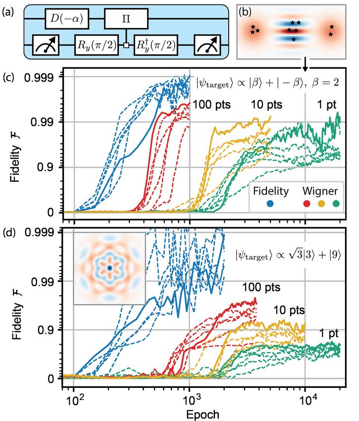
4

K[a] consists of two Kraus operators K± [a] satisfying the       tion III A. Nevertheless, it is amenable to the same solu-
                             †             †                     tion methods as classical MDPs. In the following Section,
completeness relation K+       [a]K+ [a]+K−  [a]K− [a] = I and
corresponding to observations ±1. If the control circuit         we describe a model-free RL approach to solving MDPs.
does not contain a measurement, then the map consists
of a single unitary operator K0 [a].
   4. State transitions happen deterministically accord-              C.   Policy gradient reinforcement learning
ing to |st+1 i = K0 [at ]|st i if the control circuit does not
contain a measurement, and otherwise stochastically ac-             The solution to a partially-observable MDP is a pol-
                                       √
cording to |st+1 i = K± [at ]|st i/ p± with probabilities        icy π(at |ht ) which assigns a probability distribution over
            †
p± = hst |K±  [at ]K± [at ]|st i.                                actions to each possible history ht = o0:t that the agent
   In this paper, we do not consider the coupling of a           might see. In large problems, it is unfeasible to represent
quantum system to a dissipative bath, but it can be incor-       the policy as a lookup table, and instead it is convenient
porated into the QOMDP by expanding the Kraus maps               to parameterize it using a powerful function approxima-
to include uncontrolled quantum jumps of the state |st i         tor such as a deep neural network [13, 15, 57]. As an
induced by the bath. This would lead to more compli-             additional benefit, this representation allows the learn-
cated dynamics, but since the quantum state and its tran-        ing agent to generalize via parameter sharing to histories
sitions are hidden from the agent, nothing will change in        it has never encountered during training. We will refer
the RL framework.                                                to such neural network policies as πθ where θ represents
   In the traditional approach to quantum control, the           the network parameters. It is common to adopt recur-
model for K[a] is specified, for example through the sys-        rent network architectures, such as the Long Short-Term
tem’s Hamiltonian and Schrödinger equation, allowing             Memory (LSTM) [58, 59], in problems with variable-
for gradient-based optimization of the cost function. In         length inputs. In this work, we use neural networks with
contrast, in our approach the Kraus map K[a] is not mod-         an LSTM layer and several fully connected layers.
eled. Instead, the experimental apparatus implements                The output of the policy network is not the action at
K[a] exactly. In this case, the optimization proceeds at         but the mean µθ [ht ] and variance σθ2 [ht ] of the normal
a higher level, without direct access to the gradient, but       distribution from which the action at is sampled. The
by trial-and-error learning of the patterns in the action-       stochastisity of the policy during the training ensures a
reward relationship. This ensures that the learned con-          balance between exploration of new actions and exploita-
trol sequence is free of model bias.                             tion of the current best estimate µθ of the optimal action.
   In practice, common contributions to model bias come          Typically, as training progresses the agent learns to re-
from frequency- and power-dependent pulse distortions            duce the variance σθ2 of the stochastic policy and even-
in the control lines [55, 56], higher order nonlinearities,      tually converges to a near-deterministic policy. After the
coupling to spurious modes, etc. Simulation-based ap-            training is finished, the deterministic policy is obtained
proaches often attempt to compensate for model bias by           by always choosing the optimal action µθ .
introducing additional terms in the cost function, such             Policy gradient reinforcement learning [11, 12] provides
as penalties for pulse power and bandwidth, weighted             a set of tools for learning the policy parameters θ guided
with somewhat arbitrarily chosen coefficients. In con-           by the reward signal. Even though the reward R is a
trast, our RL agent will learn the relevant constraints          non-differentiable random variable sampled from episodic
automatically, since it optimizes the true unbiased ob-          interactions with the environment, its expectation J de-
jective incorporated into the reward.                            pends on the policy parameters θ and is therefore differ-
   As shown in Fig. 1, the reward is produced by follow-         entiable. The basic working principle of the policy gra-
ing the training episode with the reward circuit. This cir-      dient algorithms is to construct an empirical estimator
cuit necessarily contains an ancilla measurement whose           gk of the gradient of performance measure ∇θ J(πθ )|θ=θk
binary outcome probabilistically indicates whether the           based on a batch of B episodes of experience collected
applied control sequence implements the desired quan-            in the environment following the current policy πθk , and
tum operation. Since the reward measurement in gen-              then performing a gradient ascent step on the policy pa-
eral will disrupt the quantum state, we only apply the           rameters θk+1 = θk + αgk , where α is the learning rate.
reward circuit at the end of the episode, and use the            This data collection and the subsequent policy update
reward rt
5
ent domains, it significantly improves learning stability,
which is especially important in stochastic environments,
motivating our choice of this learning algorithm for solv-
ing QOMDPs.
In contrast to the established gradient-based OCT
methods, in our RL approach the initial central challenge
is to achieve learning convergence at all, i.e. to ensure
that the agent’s performance gradually improves to a de-
sired level and does not collapse or stagnate. Therefore,
the majority of Section IV will be devoted to showing the
solution to this challenge on various state preparation in-
stances.
IV. Results
Currently, direct pulse shaping with GRAPE (gradi-
ent ascent pulse engineering) is a dominant approach to
quantum state preparation [45, 46, 62]. Nevertheless,
a modular approach based on repetitive application of
a parametrized control circuit has several advantages. FIG. 2. Preparation of Fock states |1i, ..., |10i. (a)
Firstly, thanks to a reduced number of parameters, the Parametrized control circuit (pink), and Fock reward circuit
modular approach is less likely to overfit and can gener- (blue). The reward circuit contains a selective π-pulse on the
alize better under small environment perturbations. In qubit, conditioned on having n photons in the oscillator. (b)
addition, each gate in the module can be individually Evaluation of the training progress. The background trajec-
tested and calibrated, further facilitating the reduction tories correspond to 6 random seeds for each state, solid lines
of bias. Finally, the modular approach is more inter- show the trajectory with the highest final fidelity.
pretable, even allowing for analytic sequence construc-
tion in special cases.
Our RL approach is compatible with any parametrized even when they do not produce the expected effect, tai-
control circuit and with the direct pulse-shaping. In loring the learned actions to the unique control imperfec-
this work, for concreteness, we made a particular choice tions present in the system. We focus on this aspect in
of a universal gate set based on the selective number- Section IV D by training the agent with an imperfectly
dependent arbitrary phase SNAP(ϕ) gate combined with implemented SNAP gate. Moreover, the advantage of
displacements D(α) [63, 64]: RL compared to other model-free optimization methods
is that it can efficiently solve problems requiring adap-
∞
X tive decision-making. A demonstration of this point for
SNAP(ϕ) = eiϕn |nihn|, (1) quantum error correction is presented in Ref. [32]. We
n=0 leverage this advantage of RL in Section IV D to find
D(α) = exp(αa† − α∗ a). (2) model-free adaptive measurement-based quantum feed-
back strategies that compensate for imperfect SNAP im-
Recently it was demonstrated that SNAP can be made plementation.
first-order path-independent with respect to ancilla qubit
decay [65, 66]. Furthermore, a linear scaling of the cir-
cuit depth T with the state size hni can be achieved for
this approach [67], while many interesting experimentally A. Preparation of oscillator Fock states
achievable states can be prepared with just T ∼ 5. In-
spired by this finding, we parametrize our open-loop con- The central question in our reinforcement learning ap-
trol circuit as D† (α) SNAP(ϕ) D(α), see Fig. 2(a). proach is how to assign a reward to the agent with-
In the following Sections IV A-IV C our aim is to out having access to the quantum state. The true op-
demonstrate that model-free reinforcement learning from timization objective is the fidelity to the target state
scarce binary reward signals in quantum-observable en- F = |hψ|ψtarget i|2 , and thus it is desirable to measure the
vironments is feasible, i.e. the learning converges to observable corresponding to the target projector. Such
high-fidelity protocols in a realistic number of training luxury is not always available in the experiment, but in
episodes. To isolate the learning aspect of the prob- the case of Fock states the projectors |nihn| can be rou-
lem, in Sections IV A-IV C we use perfect gate imple- tinely measured with a qubit coupled to the oscillator
mentations acting on the Hilbert space as intended by in the dispersive-strong regime by selectively addressing
Eqs. (1)-(2). However, the major power of the model- the number-split qubit transitions [68]. Therefore, we
free paradigm is the ability to utilize available controls use the Fock reward circuit shown in Fig. 2(a) to learn6
preparation of such states. can be periodically interleaved with evaluation epochs to
All reward circuits considered in this work contain two perform reliable state certification for the deterministic
ancilla measurements. If the SNAP is ideal as in Eq. (1), version of the current policy. Other metrics can also be
the qubit will remain in |gi after the control sequence, used to monitor the training progress without interrup-
and the outcome of the first measurement will always be tion, such as the moving average of the return of the
m1 = 1, which is the case in Sections IV A-IV C. How- stochastic policy or the entropy of the stochastic policy.
ever, in a real experimental setup, residual entanglement The agent benchmarking results for this QOMDP are
between the qubit and oscillator can remain. Therefore, shown in Fig. 2(b). It is worth pointing out yet an-
in general the first measurement serves to disentangle other difference compared to classic benchmarking en-
them. The second measurement with outcome m2 is used vironments used by the RL community [12]: in the state
to produce the reward. In the Fock reward circuit, this preparation QOMDP, the agent is required to approach
is done according to the rule R = −m2 . The expectation arbitrarily close to the maximally achievable return of
of such reward E[R] = 2Fn − 1 is proportional to the Jmax = 1. In the late stages of learning, performance
fidelity Fn = |hψ|ni|2 of the state preparation policy. is exponentially sensitive to small changes is the policy,
The training episodes begin with the oscillator in vac- which seems to require a reward signal of high resolution
uum |ψ0 i = |0i and the ancilla qubit in the ground and a learning algorithm of high stability. Our proof-of-
state |gi. Episodes follow the general template shown principle demonstration indicates that the agent is able
in Fig. 1(a), in which the control circuit is applied for to solve such QOMDPs efficiently and converge to proto-
T = 5 time-steps, followed by the Fock reward circuit. cols with F > 0.99 even when guided by low-resolution
The SNAP gate is truncated at Φ = 15 levels, leading to rewards of ±1. Further speedups in convergence and fi-
the (15 + 2)-dimensional parameterization of the control delity improvements could be possible upon hyperparam-
circuit. In our approach, the choice of the circuit depth eter optimization.
T and the action space dimension |A| = Φ + 2 needs to Arguably, under quantum observability the most ef-
be made in advance, which requires some prior under- ficient learning for the problem of state preparation is
standing of the problem complexity. In this example, we achieved when the target projector is directly measur-
chose T = 5 and Φ = 15 for all Fock states |1i,..,|10i to able. This is also the case for which there already exist
ensure a fair comparison of the convergence speed, but, experimental in-situ pulse shaping demonstrations using
in principle, the states with lower n can be prepared with randomized benchmarking to obtain the cost function for
shorter sequences [63, 64]. An automated method for se- other gradient-free optimization techniques [7–9]. But
lecting the circuit depth was proposed in Ref. [67], and how can we train the agent to prepare a state whose
it can be utilized here to make an educated guess of T . projector is not measurable within a given experimental
The action-vectors are sampled from the normal dis- platform? Before tackling this problem for the most gen-
tribution produced by the deep neural network with one eral case, we consider an intermediate-difficulty problem
LSTM layer and two fully-connected layers, representing of the stabilizer state preparation.
the stochastic policy. The neural network input is only
the “clock” observation (one-hot encoding of the step in-
dex t), since there are no measurements in the open-loop B. Preparation of stabilizer states
control circuit. The agent is trained for 4000 epochs with
batches of B = 1000 episodes per epoch. The total time The class of stabilizer states is of particular interest
budget of the training is split between (i) experience col- for quantum error correction [71]. A state |ψi is a sta-
lection, (ii) optimization of the neural network, and (iii) bilizer state if it is a 1-dimensional subspace satisfying
communication and instruments re-initialization. We es- Sk |ψi = (+1)|ψi for k = 1, ..., K, where Sk are the sta-
timate that with the help of active oscillator reset [69] the bilizer group generators, simply referred to as stabilizers.
experience collection time in experiment can be as short If all the stabilizers Sk are measurable but the state pro-
as 10 minutes in total for such training (assuming 150 µs jector |ψihψ|target is not, we can still train the agent using
duty cycle per episode). Our neural network is imple- stabilizer measurement outcomes as rewards.
mented with TensorFlow [70] on an NVIDIA Tesla V100 To demonstrate learning stabilizer state preparation,
graphics processing unit (GPU). The total time spent we train the agent to prepare a grid state, also known as
updating the neural network parameters is 10 minutes the Gottesman-Kitaev-Preskill (GKP) state [72]. Grid
in total for such training, and is expected to further re- states were originally introduced for encoding a 2D qubit
duce as GPU performance continues to improve. The real subspace into an infinite-dimensional Hilbert space of an
experimental implementation will likely be limited by in- oscillator for bosonic quantum error correction, and were
strument re-initialization [9]. This time budget puts our subsequently recognized to be valuable resources for var-
proposal within the reach of current technology. ious other quantum applications. In particular, the 1D
Throughout this manuscript, we use the fidelity F as version of the grid state which we will consider here, can
an evaluation metric to benchmark the agent, but it will be
√ used for sensing both position and momentum modulo
not be directly available in the real experimental imple- π simultaneously [73, 74].
mentation. If desired, in practice the training epochs An ideal (infinite-energy) 1D grid state is a Dirac7
√
comb |ψ0GKP i ∝
P
t∈Z D(t π)|0x i, where |0x i is a po-
sition eigenstate located at x√ = 0. The stabilizers √ of
such a state are Sx,0 = D( π) and Sp,0 = D(i π).
GKP
The finite-energy version of this state |ψ∆ i can be
−1
obtained with the stabilizers Sx,∆ = E∆ Sx,0 E∆ and
−1 2 †
Sp,∆ = E∆ Sp,0 E∆ , where E∆ = exp(−∆ a a) is the
envelope operator. The parameter ∆ defines the degree
of squeezing in the peaks of the Dirac comb and the ex-
tent of the grid envelope.
The ideal stabilizers Sx/p,0 are unitary and can be
measured in the oscillator-qubit system with the stan-
dard phase estimation circuit [75], as was experimen-
tally demonstrated with trapped ions [76] and super-
conducting circuits [77]. On the other hand, the finite-
energy stabilizers Sx/p,∆ are not unitary nor Hermi-
tian. Recently, an approximate circuit for generalized
measurement of Sx/p,∆ was proposed [78, 79] and real-
ized with trapped ions [79]. Our stabilizer reward cir-
cuit, shown in Fig. 3(a), is based on these proposals.
In this circuit, the direction of the stabilizer displace- FIG. 3. Preparation of grid states. (a) Stabilizer reward
ment (along x or p quadrature) is selected at random in circuit for the target state |ψ∆
GKP
i. The circuit makes use of
each episode. The measurement outcome m2 is adminis- the conditional displacement gate CD(α) = D(σz α/2). The
control circuit is the same as in Fig. 2(a). (b) Evaluation
tered as a reward R = m2 , which satisfies the condition
of the training progress. The background trajectories corre-
E[R] = (hSx,∆ i + hSp,∆ i)/2. The agent that strives to spond to 6 random seeds for each state, solid lines show the
maximize such a reward will learn to prepare an approx- trajectory with the highest final stabilizer value. Inset: ex-
GKP
imate |ψ∆ i state. ample Wigner functions of the states prepared by the agent
after 10,000 epochs of training.
pGrid states have a large photon number variance
var(n) = hni = 1/(2∆2 ). Therefore, the preparation
of such states requires large SNAP truncation Φ, but the
increased action space dimension |A| = Φ + 2 can result
in less stable and efficient learning. As a compromise,
we consider policies with Φ = 30 and T = 9. The list of C. Preparation of arbitrary states
other training hyperparameters is included in the Sup-
plementary Material [61].
The agent benchmarking results for this QOMDP are In the general case, we need to construct an unbi-
shown in Fig. 3(b), with average stabilizer value as the ased estimator of the fidelity F based on a measure-
evaluation metric. For a perfect policy, the stabilizers ment scheme which is tomographically complete and fea-
would saturate to +1, but it is increasingly difficult to sible to implement in a given experimental platform. In
satisfy this requirement for target states with smaller the strong dispersive limit of circuit QED it is possi-
∆ due to a limited SNAP truncation and circuit depth. ble to implement a high-fidelity measurement of pho-
†
Nevertheless, the agent successfully copes with this task. ton number parity operator Π = eiπa a , which can be
Example Wigner functions of the states prepared by the used to perform Wigner function tomography according
agent after 10,000 epochs of training are shown as insets. to W (α) = π2 hD(α)ΠD† (α)i [80]. Therefore, in princi-
ple the fidelity can be computed after tomographic re-
We conjecture that learning state preparation from sta- construction of the quantum state, and then used as a
bilizer measurements as described in this Section is more reward, although such an approach would be extremely
difficult than from target projector measurements, since sample inefficient. Fortunately, with stochastic gradi-
individual reward bits carry less information. If the sta- ent ascent, a useful policy update can be applied even
bilizer measurements can be realized in a quantum non- without knowing the exact direction of the gradient, as
demolition way, this opens the possibility of acquiring long as it generally moves the policy in the correct di-
the values of multiple commuting stabilizers after every rection. This insight motivates using noisy small-sample
episode, and thereby increasing the signal-to-noise ratio estimates of F as a reward, allowing to drastically re-
(SNR) of the reward signal. duce the sample complexity of expensive real-world RL
Examples in Sections IV A-IV B exploit the structure training.
of the problem to construct reward circuits for special
classes of states. Next, we consider how to construct a To derive an efficient reward function for arbitrary
reward circuit for preparation of arbitrary states. states, we first compute the fidelity with Monte Carlo8
Appendix A. Such a choice also helps to stabilize the
learning algorithm, since it conveniently leads to rewards
of equal magnitude (see below).
In each individual episode, we first generate the phase
space point α with rejection sampling, as illustrated in
Fig. 4(b), and then measure parity in the displaced state,
corresponding to the Wigner reward circuit shown in
Fig. 4(a). The reward is then assigned according to the
rule
R = Πα sgn Wtarget (α). (5)
This reward is equal to ±1 in each episode, and it satisfies
the requirement F ∝ E[R]. Therefore, the RL agent that
learns to achieve higher rewards, will tend to find proto-
cols with higher fidelity. Note the remarkable savings in
sample complexity: in principle, we only require a single
binary tomography measurement per policy candidate.
We emphasize that this sample efficiency is a crucial in-
novation which ensures that reinforcement learning can
be feasible to implement in real experimental systems. A
similar fidelity estimator is obtained in Appendix B for
the oscillator characteristic function which is also mea-
surable in circuit QED [77] and in trapped ions [76, 81],
and for multi-qubit characteristic function, so our ap-
proach is widely applicable.
FIG. 4. Preparation of arbitrary states. (a) Wigner reward We investigate the agent’s performance with Wigner
circuit based on the measurement of the photon number par- reward circuit for (i) preparation of the Schrödinger cat
ity. In this circuit, the conditional parity gate corresponds state |ψtarget i ∝ |βi + | − βi with β = 2 in T = 5 steps,
to |gihg| ⊗ I + |eihe| ⊗ Π. (b) Wigner function of the cat shown in Fig. 4(c), and√(ii) preparation of the binomial
state |ψtarget i ∝ |βi + | − βi with β = 2. Scattered stars code state |ψtarget i ∝ 3|3i + |9i [82] in T = 8 steps,
illustrate phase space sampling of points α for the Wigner shown in Fig. 4(d). In contrast to the target projector
reward. (c) Evaluation of the training progress for the cat and stabilizer rewards, the Wigner reward (5) will con-
state. The background trajectories correspond to 6 random tain sampling noise even under the perfect policy. Since
seeds for each setting, solid lines show the trajectory with
in this case it is not possible to find the policy that would
the highest final fidelity. The Wigner reward is obtained by
sampling 1, 10, 100 different phase space points, doing a single systematically produce the reward of +1, the agent con-
measurement per point and averaging the obtained measure- verges to policies of intermediate fidelity (green). To in-
ment outcomes to improve the resolution and achieve higher crease the SNR of the Wigner reward, we evaluate each
convergence ceiling. For blue curves the fidelity F is used as a stochastic policy realization with reward circuits corre-
reward, representing the expected performance in the limit of sponding to 1, 10, 100 different phase space points, doing
infinite averaging. (d) Evaluation of√ the training progress for a single measurement per point and averaging the ob-
the binomial code state |ψtarget i ∝ 3|3i + |9i, whose Wigner tained measurement outcomes to generate the reward R.
function is shown in the inset. The results show that increased reward SNR allows to
reach higher fidelity, albeit at the expense of increased
importance sampling of the phase space sample complexity. We expect that in the limit of infi-
Z nite averaging the training would proceed as if the fidelity
F was directly available to be used as reward (blue).
F = π d2 α W (α)Wtarget (α) (3)
This demonstration proves that arbitrary state prepa-
1
ration is in principle possible with our approach. How-
=2 E E Πα Wtarget (α) , (4) ever, we observe notable variations in convergence speed
α∼P Πα ∼ψ P (α)
and saturation fidelity depending on the choice of hyper-
where Πα ≡ m2 is a random outcome of the parity mea- parameters, which is typical of reinforcement learning. A
surement made in the state |ψi displaced by −α. The lot of progress has been made in developing robust RL
points α are sampled according to an arbitrary prob- algorithms applicable to a variety of tasks without exten-
ability distribution P (α) which is nonzero everywhere sive problem-specific hyperparameter tuning [14, 15], but
where Wtarget (α) 6= 0. The estimator (4) is unbiased this still remains a major open problem in the field. The
for any P (α), but its variance can be significantly re- list of hyperparameters used in all our training examples
duced by choosing P (α) appropriately. The lowest vari- can be found in the Supplementary Material [61].
ance is achieved with P (α) ∝ |Wtarget (α)|, as shown in Having demonstrated how to learn arbitrary state9
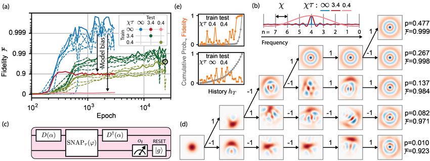
FIG. 5. Learning adaptive measurement-based quantum feedback for preparation of Fock state |3i with imperfect controls.
(a) Evaluation of the training progress. Blue: training the agent with the open-loop control circuit, shown in Fig. 2(a),
that uses an ideal SNAP – an example of model-based optimization. The background trajectories correspond to 6 random
seeds. The protocols of the best-performing seed are then tested using the same control circuit, but with a finite-duration
gate SNAPτ substituted instead of an ideal SNAP. Such a test reveals the degradation of performance (red, pink) due to the
model bias. (b) Spectrum of partially-selective qubit pulses used in the gate SNAPτ . The degradation of performance in
(a) occurs because the pulse overlaps in the frequency domain with unintended number-split qubit transitions, leaving the
qubit and oscillator entangled after the gate. (c) Closed-loop control circuit containing a finite-duration gate SNAPτ and a
verification measurement that produces an observation ot and disentangles qubit and oscillator. The qubit is always reset to
|gi after the measurement. This control circuit requires either post-selection or adaptive control. The agent successfully learns
measurement-based feedback control (a, green) even in the extreme case χτ = 0.4 far from theoretically optimal regime χτ
1.
(d) An example state evolution under the policy obtained after 25,000 epochs of training, shown with a black circle in (a).
The agent chooses to focus on a small number of branches and ensure that they lead to high-fidelity states. (e) Cumulative
probability and fidelity of the observed histories quantifies this trend (top panel). The policy trained with ideal SNAP and
tested with SNAPτ (bottom panel) has relatively uniform probability of all histories and poor fidelity.
preparation, we next move on to an example highlighting leave the qubit and oscillator entangled. Such imperfec-
the benefits of model-free (as opposed to model-based) tions are notoriously difficult to calibrate out or precisely
learning and the potential of RL for measurement-based account for at the pulse or sequence construction level,
feedback control. which presents a good testbed for our model-free learn-
ing paradigm. We demonstrate that our approach leads
to high-fidelity protocols even in the case τ < 1/χ far
D. Learning adaptive quantum feedback with from theoretically optimal regime, where the sequences
imperfect controls. produced assuming ideal SNAP yield poor fidelity due to
severe model bias.
In the oscillator-qubit system with dispersive coupling We begin by illustrating in Fig. 5(a) the degradation
Hc /h = 12 χ a† a σz , the Berry phases ϕn in (1) are created of performance of the policies optimized for Fock state
through qubit rotations: |3i preparation using the open-loop control circuit from
SNAP(ϕ) =
X
|nihn| ⊗ Rπ−ϕn (π)R0 (π), (6) Fig. 2(a) with an ideal SNAP (blue), when tested with a
n
finite-duration gate SNAPτ (red, pink) whose details are
included in the Supplementary Material [61]. Achieving
where Rφ (ϑ) = exp(−i ϑ2 [cos φ σx +sin φ σy ]). Such an im- extremely high fidelity (blue) requires delicate adjust-
plementation relies on the ability to selectively address ment of the control parameters, but this fine-tuning is
number-split qubit transitions, which requires pulses of futile when the remaining infidelity is smaller than the
long duration τ
1/χ. In practice, it is desirable to keep model bias. As seen by testing on the χτ = 3.4 case
the pulses short to reduce the probability of ancilla relax- (red), any progress that the optimizer made after 300
ation during the gate. However, shorter pulses of wider epochs was due to overfitting to the model of the ideal
bandwidth would drive unintended transitions, as illus- SNAP. As depicted with a spectrum in Fig. 5(b), the
trated in Fig. 5(b), leading to imperfect implementation qubit pulse of such duration is still reasonably selective
of the SNAP gate: in addition to accumulating incor- (and is close to the experimental choice χτ ≈ 4 in [64]),
rect Berry phases for different levels, this will generally but it already requires a much more sophisticated mod-10 eling of the SNAP implementation in order to not limit of which yield F > 0.9, and further post-selection of his- the experimental performance. In the partially selective tory hT = 11111 will boost the fidelity to F > 0.999. We case χτ = 0.4 (pink) the performance is drastically worse. observe that fidelity reduces in the branches with more Note that optimization with any other simulation-based “-1” measurement outcomes (top to bottom), because, approach assuming ideal SNAP, such as [63, 67], would being less probable, such branches receive less attention exhibit a similar degradation. from the agent during the training. As shown in Fig. 5(e) One way to recover higher fidelity is through a detailed top panel, the agent chooses to focus on only a small num- modeling of the composite qubit pulse in the SNAP [83], ber of branches and ensure that they lead to high-fidelity although such approach will still contain residual model states. This is in contrast to the protocol optimized with bias. An alternative approach, which comes at the ex- the ideal SNAP and tested with SNAPτ (bottom panel), pense of reduced success rate, is to perform a verification which, as a result of model bias, performs poorly and has ancilla measurement and post-selection, leading to a con- relatively uniform probability of all histories (of course, trol circuit shown in Fig. 5(c). Post-selecting on a qubit such protocol would produce only 11111 if it was applied measured in |gi in all time steps (history hT = 11111) with ideal SNAP). significantly boosts the fidelity of a biased policy from It is noteworthy that in the two most probable 0.9 to 0.97 in the case χτ = 3.4, but does not lead to any branches in Fig. 5(e) the agent actually finishes prepar- improvement in the extreme case χτ = 0.4. The post- ing the state in just 3 steps, and in the remaining time selected fidelity is still lower than with the ideal SNAP, chooses to simply idle instead of further entangling the because this scheme only compensates for qubit under- or qubit with the oscillator and subjecting itself to addi- over-rotation, and not for the incorrect Berry phases. Ad- tional measurement uncertainty. In the other branches, ditionally, the trajectories corresponding to other mea- this extra time is used to catch up after previously re- surement histories have extremely poor fidelities because ceiving undesired measurement outcomes. This indeed only the history hT = 11111 was observed during the op- seems to be an intelligent strategy for such a problem, timization with an ideal SNAP. However, in principle, if which serves as a positive indication that such agent will the qubit is projected to |ei by the measurement, the de- be able to cope with incoherent errors by shortening the sired state evolution can still be recovered using adaptive effective sequence length. quantum feedback. A general policy in such setting is a We emphasize that even though for the simulated binary decision tree of depth T , equivalent to 2T −1 dis- demonstration of model-free learning we had to build tinct parameter settings for every possible measurement a specific model of the finite-duration qubit pulse, the history. There exist model-based methods for construc- agent is completely agnostic to it by construction. The tion of such a tree [84], but they are not applicable in the only input that the agent receives is binary measurement cases dominated by a-priori unknown control errors. An outcomes, and the source of these bits is a black box to RL agent, on the other hand, can discover such a tree in a the agent. Effectively, in this demonstration the model model-free way. Even though our policies are represented bias comes from the mismatch between ideal and finite- with neural networks, they can be easily converted to a duration SNAP. We also tested the agent against other decision tree representation which is more advantageous types of model bias, such as random static offsets added for low-latency inference in real-world experimental im- to the Berry phases or qubit rotation angles, and found plementation. that the agent performs equally well in these situations. To this end, we train a new agent with a closed-loop control circuit that directly incorporates a finite-duration imperfect gate SNAPτ , shown in Fig. 5(c), mimicking training in an experiment. We use Fock reward circuit, V. Discussion shown in Fig. 2(a), in which m1 = 1 in all episodes de- spite the imperfect SNAP because of the qubit reset oper- ation. Since the control circuit contains a measurement, A natural question to ask is whether our approach will the agent will be able to dynamically adapt its actions de- scale favorably with increased (i) target state complexity, pending on the received outcomes ot . As shown with the (ii) action space dimension, (iii) sequence length. green curves in Fig. 5(a), the agent successfully learns (i) Target state complexity. Sample efficiency of adaptive strategies of high fidelity even in the extreme learning the control policy is affected by multiple in- case χτ = 0.4. This demonstrates that RL is not only teracting factors, but among the most important is the good for fine-tuning or “last-mile” optimization, but is a variance of the fidelity estimator used for the reward as- valuable tool for the domains where model-based quan- signment. The variance of the estimator in Eq. (4) with tum control completely fails due to model inadequacy. P (α) ∝ |WtargetR(α)| is given by Var = 4(1+δtarget )2 −F 2 , To further analyze the agent’s strategy, we select the where δtarget = |Wtarget (α)|dα − 1 is one measure of the best-performing random seed for the case χτ = 0.4 after state non-classicality known as the Wigner negativity [85] 25,000 epochs of training and visualize the resulting state (see Appendix A for the derivation). This result leads to evolution in Fig. 5(d). The average fidelity of such policy a simple lower bound on the sample complexity of learn- is F = 0.974. There are 5 high-probability branches, all ing the state preparation policy that reaches the fidelity
11

F to the desired target state                                    ability that are not specific to quantum control, but are
                                                                 common in any control task. The generality of the model-
                      4(1 + δtarget )2 − F 2                     free reinforcement learning framework makes it possible
                M>                           .            (7)
                           (1 − F)2                              to transfer the solutions to such challenges, found in other
                                                                 domains, to quantum control problems.
This expression bounds the number of measurements M
required for the state certification alone, i.e. for resolving      Let us now return to the discussion of other factors in-
the fidelity F of a fixed policy with statistical uncertainty    fluencing the sample efficiency. As we briefly alluded to
comparable to the infidelity. The task of the RL agent           previously, the overhead on top of Eq. (7) depends on the
is more complicated, since it needs to not only resolve          learning algorithm and its hyperparameters. Model-free
the fidelity of the current policy, but also learn how to        RL is known to be less sample efficient than gradient-
improve it. Therefore, this bound is likely not tight, and       based methods, typically requiring millions of training
the practical overhead depends strongly on the learning          episodes [12]. On-policy RL algorithms, such as PPO, are
algorithm and its hyperparameters (we will return to the         among the least sample efficient, since they discard the
topic of how these factors influence the sample efficiency       training data after each policy update. In contrast, off-
shortly). However, the bound (7) clearly indicates that          policy methods keep old experiences in the replay buffer
learning the preparation of non-classical states is increas-     and learn from them even after the current policy has
ingly difficult, as one would expect, and the difficulty can     long diverged from the old policy under which the data
be quantified according to the Wigner negativity of the          was collected, typically resulting in better sample effi-
state. This is a fundamental limitation on the learning          ciency. Our pick of PPO was motivated by its simplicity
efficiency which can only be overcome by taking advan-           and stability in the stochastic setting, but it is worth
tage of the special structure of the states and available        exploring an actively expanding collection of RL algo-
measurements, as we did, for instance, for Fock states           rithms [12], and understanding which are most suitable
and GKP states.                                                  for quantum-observable environments.
   (ii) Action space dimension.The practical overhead               The sample efficiency of model-free RL in the quantum
on top of Eq. (7) is determined, among other factors,            control setting can be further improved by utilizing the
by the choice of the control circuit. Operating with             strength of conventional OCT methods. A straightfor-
SNAP and displacements, the action space dimension               ward way to achieve this would be through supervised
|A| = Φ + 2 will have to grow with the target state              pre-training of the agent’s policy in the simulation. Such
size to ensure individual control of the phases of involved      pre-training would provide a better starting point for the
oscillator levels. This might be problematic, since the          agent subsequently re-trained in the real-world setting.
performance of RL (or any other approach) is generally           Our preliminary numerical experiments show that this
worse on high-dimensional tasks, as evidenced, for in-           indeed provides significant speedups.
stance, by studies of robotic locomotion with different             The proposals discussed above resolve the bias-
numbers of controllable joints [86, 87]. Our modular ap-         variance trade-off in favor of complete bias elimination,
proach allows for an alternative solution of adopting a          necessarily sacrificing sample efficiency. In this respect,
different control circuit, necessarily trading the action        model-free learning is a swing in the opposite direction
space dimensionality |A| for the sequence length T . For         from the traditional approach in physics of constructing
example, conditional displacements and qubit rotations           sparse physically-interpretable models with very few pa-
[88] form another gate set for the universal control of          rameters which can be calibrated in experiment. Building
an oscillator, whose dimensionality |A| = 4 is target-           on the insights from machine learning community, model
state-independent. Distributing the problem complexity           bias can in principle be strongly reduced (not eliminated)
between |A| and T in the optimal way requires consider-          by learning a richly parametrized model, either physi-
ation of various tradeoffs involving both the properties of      cally motivated [90, 91] or neural-network-based [92, 93],
the quantum environment and capabilities of the agent.           from direct interaction with a quantum system on which
   (iii) Sequence length. Tackling decision-making               the control policy is ultimately to be deployed. The
problems with long-term dependencies (i.e. T  1) is             learned model can then be used to optimize the con-
what made RL popular in the first place, as exemplified          trol policy with simulation-based (not necessarily RL)
by various game-playing agents [13–16]. In quantum con-          methods. Another promising alternative is to use model-
trol, the temporal structure of the control sequences can        based reinforcement learning techniques [94], where the
be exploited by adopting recurrent neural network archi-         agent can plan the actions by virtually interacting with
tectures, such as the LSTM used in our work. Recently,           its learned model of the environment while refining both
machine learning for sequential data has significantly ad-       the model and the policy using real-world interactions.
vanced with the invention of the Transformer models [89]         In particular, the MuZero algorithm [95], a descendant of
which use attention mechanisms to ensure that the gra-           AlphaGo [13], is combining model learning and planning
dients do not decay with the sequence depth T . Machine          with Monte Carlo tree search to achieve state-of-the-art
learning innovations such as this will undoubtedly find          performance on diverse tasks, and holding great promise
applications in quantum control.                                 for quantum control. Finally, in addition to adopting
   As can be seen above, there are some aspects of scal-         existing RL algorithms, a worthwhile direction is to de-
You can also read