Modeling Dynamic Hair as a Continuum
←
→
Page content transcription
If your browser does not render page correctly, please read the page content below
EUROGRAPHICS 2001 / A. Chalmers and T.-M. Rhyne                                                                             Volume 20 (2001), Number 3
(Guest Editors)

                              Modeling Dynamic Hair as a Continuum

                                                         Sunil Hadap and Nadia Magnenat-Thalmann

                                                               {sunil,nadia}@miralab.unige.ch
                                                         MIRALab, CUI, University of Geneva, Switzerland
                                                                 http://www.miralab.unige.ch/

         Abstract
         In this paper we address the difficult problem of hair dynamics, particularly hair-hair and hair-air interactions.
         To model these interactions, we propose to consider hair volume as a continuum. Subsequently, we treat the
         interaction dynamics to be fluid dynamics. This proves to be a strong as well as viable approach for an otherwise
         very complex phenomenon. However, we retain the individual character of hair, which is vital to visually realistic
         rendering of hair animation. For that, we develop an elaborate model for stiffness and inertial dynamics of
         individual hair strand. Being a reduced coordinate formulation, the stiffness dynamics is numerically stable and
         fast. We then unify the continuum interaction dynamics and the individual hair’s stiffness dynamics.

1. Introduction                                                                         to the previous hair dynamics attempts, mainly explicit hair
                                                                                        models. In these models, each hair strand is considered for
One of the many challenges in simulating believable virtual
                                                                                        shape and dynamics. That makes explicit models tedious
humans and animals has been to produce realistic looking
                                                                                        for shape modeling and numerically intensive for dynamics,
hair. Hair simulation can be thought of having three different
                                                                                        however they are intuitive and close to reality. They are
subtasks - shape modeling, dynamics and rendering. We
                                                                                        especially suitable for dynamics of long hair. Daldegan et
can even classify the hair modeling attempts based on their
                                                                                        al 4 and Rosenblum et al 5 used a mass-spring-hinge model
underlying models, namely explicit hair models, cluster hair
                                                                                        to control the position and orientation of hair strand. As their
models and volumetric textures. Hair rendering and shape
                                                                                        dynamic models were for straight hair, they could not be
modeling of fur like short hair is becoming increasingly
                                                                                        applied in animating hairstyles. Anjyo et al 6 modeled hair
available to animators. However, shape modeling and
                                                                                        with a simplified cantilever beam and used one-dimensional
dynamics of long hair has been difficult. The difficulties
                                                                                        projective differential equation of angular momentum to
stem from the shear number of hair strands, their geometric
                                                                                        animate hair. Although the algorithm dealt with both
intricacies and associated complex physical interactions. In
                                                                                        hairstyling and hair animation, it had several limitations, the
this paper, we concentrate on the dynamics of long hair. The
                                                                                        original hairstyle could not be recovered after subsequent
specific contributions are as follows:
                                                                                        animation and the movement of head was not accounted
• We address the problem of hair-hair, hair-body and hair-                              for. Further, the approximation in collision detection could
  air interactions. We make a paradigm shift and model                                  generate unnatural results when the algorithm was used to
  these interactions, in a unified way, as fluid dynamics.                              animate long hair. To reduce computations, Daldegan et al 4
  We use smoothed particle hydrodynamics (SPH) 1, 2 as a                                used a wisp model. Recently, Lee et al 7 developed on
  numerical model.                                                                      Anjyo’s work to add some details to model hairstyles.
• We give an elaborate model for the stiffness dynamics
                                                                                          Appreciably, none of the previous attempts considered
  of individual hair. We treat a hair strand as a serial rigid
                                                                                        hair-hair and hair-air interactions. Even individual hair
  multibody system. This reduced coordinate formulation
                                                                                        dynamics was grossly approximated to suit available
  eliminates stiff numerical equations as well as enables a
                                                                                        computational power. However, in recent years the
  parametric definition of bending and torsional dynamics.
                                                                                        computing power has grown many times. Supercomputing
  The detailed discussion on the state of the art in hair                               power of the past is becoming increasingly available to
simulation can be found in 3 . Here, we limit the overview                              animator’s workstations. There is a need to develop new hair

 c The Eurographics Association and Blackwell Publishers 2001. Published by Blackwell
Publishers, 108 Cowley Road, Oxford OX4 1JF, UK and 350 Main Street, Malden, MA
02148, USA.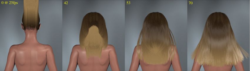
Sunil Hadap and Nadia Magnenat-Thalmann / Modeling Dynamic Hair as a Continuum

                                                                   air, as it moves it generate a boundary layer of air.
                                                                   This influences many other hair strands in motion. This
                                                                   aerodynamic form of friction is comparable to hair-hair
                                                                   contact friction. In addition, there are electrostatic forces
                                                                   to take part in the dynamics. It is not feasible to model
                                                                   these complex multiple forms of interactions. This inspires
                                                                   us to consider dynamics of single hair interacting with other
                                                                   surrounding hairs in a global manner through the continuum
                                                                   assumption. That way, we hope to have a sound model for
                                                                   an otherwise very complex phenomenon.
                                                                      As we start considering hair as a continuum, we look at
              Figure 1: Hair as a Continuum                        the properties of such a medium, namely the hair medium.
                                                                   There are two possibilities; hair medium could be considered
                                                                   as a solid or a liquid, depending on how it behaves under
dynamics models in light of current and future computing           shearing forces. Under shearing stresses, solids deform till
advances.                                                          they generate counter stresses. If the shearing stresses are
                                                                   removed, the solids exhibit ability of retaining their original
   In the next section, we develop the basic continuum             shape. The liquids are not able to withstand any shearing
hair model. Section 3 gives a detailed model of stiffness          stresses. Under the influence of the shearing stresses they
dynamics for single hair. Section 4 explains the integration       continue to deform indefinitely and they don’t have any
of two seemingly disparate approaches, hair volume as              shape memory. In case of hair, if we apply a lateral shearing
a continuum and dynamics of an individual hair. Section            motion it acts like a liquid. At the same time, length wise,
5 extends the idea of hair as a continuum to a mixture             it acts as a solid. Thus there is a duality in the behaviour of
of hair and air. Section 6 explains the implementation             hair as a continuum.
issues. Finally we show the results that demonstrate the
effectiveness of the developed hair dynamics model in                 However, from an animation point of view, we cannot
animating long hair.                                               treat hair solely as a continuum, unless the viewpoint is
                                                                   far enough and individual hair movement is not perceived.
                                                                   Thus, we have to retain the individual character of hair as
2. Hair as a Continuum                                             well, while considering hair as a continuum. We split hair
Hair-hair interaction is probably the most difficult problem       dynamics into two parts:
in achieving visually pleasing hair dynamics. So far, there        • Hair-hair, hair-body and hair-air interactions, which are
are no good models developed in this regard. Though there            modeled using continuum dynamics, and more precisely
are many advances in collision detection and response 8 ,            fluid dynamics
they are simply unsuitable for the problem at hand,                • Individual hair geometry and stiffness, which is modeled
because of shear number complexity of hair. We take a                using the dynamics of an elastic fiber
radical approach by considering hair as a continuum. The
                                                                      Interestingly, this approach even addresses the solid-
continuum assumption states that the physical properties of
                                                                   liquid duality effectively. The model can be visualized as a
a medium such as pressure, density and temperature are
                                                                   bunch of hair strands immersed in a fluid. The hair strands
defined at each and every point in the specified region. Fluid
                                                                   are kinematically linked to fluid particles in their vicinity.
dynamics regards liquids and gasses as a continuum and
                                                                   The individual hair has its own stiffness dynamics and it
even elastic theory regards solids as such, ignoring the fact
                                                                   interacts with the environment through the kinematical link
that they are still composed of individual molecules. Indeed,
                                                                   with the fluid. Density, pressure and temperature are the
the assumption is quite realistic at a certain length scale of
                                                                   basic constituents of fluid dynamics. The density of the hair
the observation but at smaller length scales the assumption
                                                                   medium is not precisely the density of individual hair. It
may not be reasonable. One might argue, hair-hair spacing
                                                                   is rather associated with the number density of hair in an
is not at all comparable to inter molecular distances to
                                                                   elemental volume. In figure 1, observe that the density of
consider hair as a continuum. However, individual hair-
                                                                   hair medium is less when the number density of hair is less.
hair interaction is of no interest to us apart from its end
                                                                   The density of the hair medium is thus defined as the mass
effect. Hence, we treat the size of individual hair and hair-
                                                                   of the hair per unit occupied volume and is denoted as ρ. The
hair distance much smaller than the overall volume of hair,
                                                                   notion of density of hair medium enables us to express the
justifying the continuum assumption. For an interesting
                                                                   conservation of mass (it is rather conservation of the number
discussion on the continuum assumption refer to 9 . As we
                                                                   of hair strands) in terms of the continuity equation 9 :
develop the model further, it will be apparent that the above
assumption is not just about approximating the complex                                    1 dρ
                                                                                               = −∇ ·~v                                     (1)
hair-hair interaction. An individual hair is surrounded by                                ρ dt

                                                                                    c The Eurographics Association and Blackwell Publishers 2001.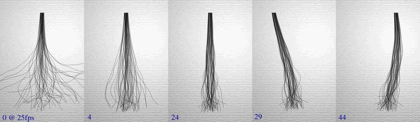
Sunil Hadap and Nadia Magnenat-Thalmann / Modeling Dynamic Hair as a Continuum
where, ~v is the local velocity of the medium. The
continuity equation states that the relative rate of change of
density ( ρ1 dρ
dt ), at any point in the medium, is equal to the
Kc
negative gradient of the velocity field at that point (−∇ ·~v). pressure
This is the total outflux of the medium at that point. The (p)
physical interpretation of the continuity equation in our case
(ρ)
is that, as the hair strands start moving apart, their number ρ0 ρc ρh hair volume density
density, and hence the density of the hair medium drops and
vice a versa.
The pressure and the viscosity in the hair medium Figure 2: Equation of State
represent all the forces due to various forms of interactions
of hair strands described previously. If we try to compress a
bunch of hair, it develops a pressure such that hair strands
physical density of hair, ρh . Figure 2 illustrates the relation
will tend to move apart. The viscosity would account for
between the density and the pressure of the hair medium. In
various forms of interactions such as hair-hair, hair-body and
the proposed pressure/density relationship, notice that there
hair-air. These are captured in the form of the momentum
is no pressure built up below the hair rest density ρ0 . As one
equation 9 of a fluid.
starts squeezing the hair volume, pressure starts building up.
d~v As a consequence, the hair strands are forced apart. At the
ρ = ν∇ · (∇~v) − ∇p + Fbd (2) hair compaction density ρc , the pressure is maximum. Kc is
dt
the compressibility of the hair volume. The power n refers
The acceleration of fluid particles d~v to the ability of hair volume to get compressed. If the hair
dt with spatial pressure
variation −∇p would be such that it will tend to even out is well aligned, the power is high. As we compress the hair
the pressure differences and as the fluid particles move, volume, suddenly hair strands start to form close packing
there will be always resistance ν∇ · (∇~v) in the form of and build the pressure quickly. On the contrary, if hair is
the friction. The body forces Fbd , i.e. the inertial forces and wavy and not very well aligned, the pressure build up is not
gravitational influence are also accounted for in the equation. abrupt.
Temperature considerably affects the properties of hair. Instead of modeling collisions of individual hair strand
However, we do not have to consider it in dynamics. We with the body, we model them, in a unified way, as boundary
treat the hair dynamics as an isothermal process unless condition of the fluid flow. There are two forms of fluid
we are trying to simulate a scenario of hair being dried boundary conditions
with a hair dryer. Secondly, the temperature is associated • Flow tangency condition - The fluid flow normal to the
with the internal energy of the fluid, which is due to the obstacle boundary is zero
continuous random motion of fluid molecules. At the length • Flow slip condition - The boundary exerts a viscous
scale of our model i.e. treating hair as a continuum, there pressure proportional to the tangential flow velocity
is no such internal energy associated with the hair medium.
Subsequently, we drop the energy equation of fluid, which is Formulation of the flow boundary condition is deferred to
associated with the temperature and the internal energy. section 4.
The equation of state (EOS) 9 binds together all the fluid
3. Single Hair Dynamics
equations. It gives a relation between density, pressure and
temperature. In our case of hair-hair interaction, EOS plays a In the previous section we discussed how we could think
central role along with the viscous fluid forces. The medium of hair-hair interaction as fluid forces by considering hair
we are modeling is not a real medium such as gas or liquid. volume as a continuum. However, for the reasons explained
Hence, we are free to "design" EOS to suit our needs: there, we still need to retain the individual character of a
hair strand. The stiffness dynamics of an individual hair is
if ρ < ρ0 ,
0
discussed in this section.
p = Kc ( ρρ−ρ 0 n
c −ρ0
) if ρ0 ≤ ρ < ρc , (3) In a very straightforward manner, one may model hair
if ρc < ρ
Kc as a set of particles connected by tensile, bending and
torsional springs 4, 5 , as shown in figure 3. If the hair strand is
We define hair rest density ρ0 as a density below which approximated by a set of n particles, then the system has 6n
statistically there is no hair-hair collision. In addition, we degrees of freedoms (DOFs) attributed to three translations,
define hair close packing density as ρc that represents the two bendings and one twist per particle. Treating each
state of the hair medium in which hair strands are packed to particle as a point mass, we can setup a set of governing
the maximum extent. This density is slightly lower than the differential equations of motion and try integrating them.
c The Eurographics Association and Blackwell Publishers 2001.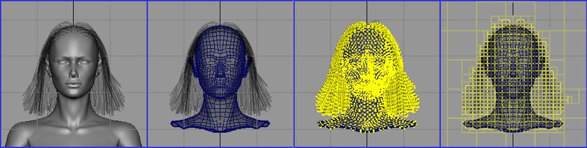
Sunil Hadap and Nadia Magnenat-Thalmann / Modeling Dynamic Hair as a Continuum

                                                                       Link 0                                   F i-1
                 Bending/Torsion         Elastic
                                                                        Link 1

      m1           m2           m1           mn-1         mn                                                       cm                i X i-1
                                                                                                                        (link-link transformation)

                                                                           Link i-1

   Figure 3: Hair Strand as an Oriented Particle System
                                                                           Link i

                                                                                                      Joint i
                                                                                                                              Fi

Unfortunately this is not a viable solution. Hair is one of               Link n

the many interesting materials in nature. It has remarkably
high Elastic Modulus of 2-6GPa. Moreover, being very
small in diameter, it has very large tensile strength when           Figure 4: Hair Strand as Rigid Multibody Serial Chain
compared to its bending and torsional rigidity. This proves to
be more problematic in terms of the numerics. We are forced
to choose very small time steps due to the stiff equations
corresponding to the tensile mode of motion, in which we           from strand to strand. The n segments are labelled as link1
are hardly interested. In fact, the hair fiber hardly stretches    to linkn . Each link is connected to two adjacent links by
by its own weight and body forces. It just bends and twists.       a three DOF spherical joint forming a single un-branched
                                                                   open-loop kinematic chain. The joint between linki−1 and
   Hence, it is better to choose one of the following two
                                                                   linki is labelled jointi . The position where the hair is rooted
possibilities. Constrain the differential motion of the
                                                                   to scalp is synonymous to link0 and the joint between head
particles that amounts to the stretching using constrained
                                                                   and hair strand is joint1 .
dynamics 10 . Alternatively, reformulate the problem
altogether to remove the DOFs associated with the                     Further, we introduce n coordinate frames Fi , each
stretching, namely a reduced coordinate formulation 11 .           attached to the corresponding linki . The coordinate frame
Both methods are equally efficient, being linear time.             Fi moves with the linki . The choice of coordinate system is
Parameterizing the system DOFs by an exact number of               largely irrelevant to the mathematical formulations, but they
generalized coordinates may be extremely hard or even              do have an important bearing on efficiency of computations,
impossible for the systems having complex topology. In this        which is discussed in Section 6. Having introduced the link
case, a constrained method is preferred for its generality         coordinates, we need to be able to transform representations
and modularity in modeling complex dynamical systems.              of the entities into and out of the link coordinates. i X̂i−1
However, for the problem at hand, the reduced coordinate           is an adjacent-link coordinate spatial transformation† which
formulation is a better method for the following reasons:          operates on a spatial vector represented in coordinate frame
• Reduced coordinates are preferred when in our case the           Fi−1 and produces a representation of the same spatial
  3n DOFs remaining in the system are comparable to the            vector in coordinate frame Fi . i X̂i−1 is composed of a pure
  3n DOFs removed by the elastic constraints.                      translation, which is constant, and a pure orientation which
• The system has fixed and simple topology where each              is variable. We use a unit quaternion qi to describe the
  object is connected to maximum of two neighbours. We             orientation. Then, we augment components of n quaternions,
  can take advantage of the simplicity and symbolically            one per joint, to form q ∈
Sunil Hadap and Nadia Magnenat-Thalmann / Modeling Dynamic Hair as a Continuum
3.2. Kinematic Equations field value A(rb)
at moving points
A 6 × 3 motion sub-space Ŝ relates the angular velocity
wi to spatial velocity across the joint, which is the only
allowed motion by the spherical joint. Since the position of
the link in its own coordinate frame remains fixed, we can field value
at grid points
express the spatial inertia Îi and the motion sub-space Ŝ as
a constant. Further, by proper choice of coordinate system,
Îi assumes a rather simple form. Subsequently, the velocity hair strands
and acceleration across the spherical joint are given by the field A(r)
following equations:
(i,j)
As(r)
v̂i = i X̂i−1 v̂i−1 + Ŝwi (4)
âi = ˆ Ŝwi + Ŝẇi
i X̂i−1 âi−1 + v̂i × (5) Figure 5: Fluid Dynamics - Eulerian and Langrangian
viewpoints
1 0 0
0 1 0
0 0 1
Ŝ =
0 0 0
• In order to account for the bending and torsional rigidity
0 0 0
of the hair strand, the jointi exerts an actuator force
0 0 0 Qai ∈Sunil Hadap and Nadia Magnenat-Thalmann / Modeling Dynamic Hair as a Continuum
the same. However, we opted for the other, less popular but
effective, Langrangian formulation of fluid dynamics.
3 2 3 3
(1 − 2 s + 4 s ) if 0 ≤ s ≤ 1,
σ 1
In Langrangian formulation, the physical properties are W (r, h) = ν 4 (2 − s)3 if 1 ≤ s ≤ 2, (13)
h
expressed as if the observer is moving with the fluid
0 otherwise
particle. Smoothed Particle Hydrodynamics (SPH) 2 is one
of the Langrangian numerical methods, that utilizes space Where s = |r|/h, ν is the number of dimensions and σ is
discretisation via number of discrete points that move with the normalization constant with values 32 , 7π10
, or π1 in one,
the fluid flow. One of the first applications of SPH in two, or three dimensions, respectively. We can see that the
computer animation was done by Gascuel et al 1 . For a good kernel has a compact support, i.e. its interactions are exactly
overview of SPH, refer 13 . zero at distances |r| > 2h. We keep the h constant throughout
Figure 5 illustrates the concept of smoothed particles. The the simulation to facilitate a speedy search of neighbourhood
physical properties are expressed at the centre of each of of the particles. The nearest neighbour problem is well
these smoothed particles. Then the physical property at any known in computer graphics. Section 6 gives the strategy
point in the medium is defined as a weighted sum of the for the linear time neighbour search.
properties of all the particles. There is no underlying grid structure in the SPH method,
which makes the scheme suitable for our purpose. We are
mb
As (r) = ∑ Ab W (r − rb , h) (8) free to choose the initial positions of the smoothed particles
b
ρb as long as their distribution reflects the local density depicted
by Equation 9. Eventually the particles will move with
The summation interpolant As (r) can be thought of as the the fluid flow. In order to establish the kinematical link
smoothed version of the original property function A(r). The between the individual hair dynamics and the dynamics of
field quantities at particle b are denoted by a subscript b. interactions, we place the smoothed particles directly onto
The mass associated with particle b is mb and density at the the hair strands as illustrated in the Figure 5. We keep the
centre of the particle b is ρb , and the property itself is Ab . We number of smoothed particles per hair segment constant, just
see that the quantity mρbb is the inverse of the number density as we have kept the hair segment length constant, for reasons
(i.e. the specific volume) and is, in some sense, a volume of computational simplicity. As the smoothed particles are
element. glued to the hair strand, they can no longer move freely with
the fluid flow. They just exert forces arising from the fluid
To exemplify, the smoothed version of density at any point
dynamics onto the corresponding hair segment and move
of medium is
with the hair segment (in the figure, the hair strand is not
discretised to show the segments). Using this method, we
ρ(r) = ∑ mbW (r − rb , h) (9) have incorporated both, the elastic dynamics of individual
b hair and the interaction dynamics into hair dynamics.
Similarly, it is possible to obtain an estimate of the Apart from providing the kinematical link, the SPH
gradient of the field, provided W is differentiable, simply by method has other numerical merits when compared to a grid-
differentiating the summation interpolant based scheme:
• As there is no need for a grid structure, we are not defining
mb
∇As (r) = ∑ Ab ∇W (r − rb , h) (10) a region of interest to which the dynamics must confine to.
b
ρb This is very useful considering the fact that, in animation
the character will move a lot and the hair should follow it.
The interpolating kernel W (r − r0 , h) has the following • No memory is wasted in defining field in the region where
properties there is no hair activity, which is not true in the case of
grid-based fluid dynamics.
• As the smoothed particles move with the flow carrying
Z
W (r − r0 , h)dr0 = 1 (11)
the field information, they optimally represent the
limW (r − r0 , h) = δ(r − r0 ) (12) fluctuations of the field. In the case of grid-based scheme,
it is necessary to opt for tedious adaptive grid to achieve
similar computational resolution.
The choice of the kernel is not important in theory as
long as it satisfies the above kernel properties. For practical In the rest of the section, we discuss the SPH versions
purposes we need to choose a kernel, which is simple to of the fluid dynamics equations. Each smoothed particle
evaluate and has compact support. The smoothing length has a constant mass mb . The mass is equal to the mass
h defines the extent of the kernel. We use the cubic spline of the respective hair segment divided by the number of
interpolating kernel. smoothed particles on that segment. Each particle carries a
c The Eurographics Association and Blackwell Publishers 2001.Sunil Hadap and Nadia Magnenat-Thalmann / Modeling Dynamic Hair as a Continuum
variable density ρb , variable pressure pb and has velocity vb . (Equation 2). Taking inputs from the artificial viscosity form
The velocity vb is actually the velocity of the point on the for SPH proposed by 13 , we set it to
hair segment where the particle is located, expressed in the ( −cµ
global coordinates. rb is the global position of the particle, ij
if µi j < 0
i.e. the particle location on the hair segment in the global ∏ =
0
ρ̄i j
if µi j ≥ 0
ij
coordinates. Once initially we place the particles on the hair
vi j · ri j
strands, we compute the particle densities using Equation 9. µi j = h
Indeed, the number density of hair at a location reflects the |ri j |2 + h2 /100
local density, which is consistent with the definition of the ρ̄i j = (ρi + ρ j )/2 (16)
density of the hair medium given in Section 2.
The constant c is the speed of sound in the medium.
For brevity, introducing notation Wab = W (ra − rb , h) and
However, in our case, it is just an animation parameter.
let ∇aWab denote the gradient of Wab with respect to ra (the
We are free to set this to an appropriate value that obtains
coordinates of particle a). Also quantities such as va − vb
satisfactory visual results. The term incorporates both bulk
shall be written as vab .
and shear viscosity.
The density of each particle can be always found from
It is quite straightforward to model solid boundaries,
Equation 9, but this equation requires an extra loop over all
either stationary or in motion, with special boundary
the particles (which means the heavy processing of nearest
particles. The boundary particles do not contribute to the
neighbour finding) before it can be used in the calculations.
density of the fluid and they are inert to the forces coming
A better formula is obtained from the smoothed version of
from the fluid particles. However, they exert a boundary
the continuity equation (equation 1).
force onto the neighbouring fluid particles. A typical form
N
of boundary force is as given in 13 . Each boundary particle
dρi
dt
= ∑ m j vi jWi j (14) has an outward pointing unit normal n and exerts a force
j=1
fn = f1 (n · 4r)P((t) · 4r)n
We now can update the particle density without going ft = K f (t · 4v)t (17)
through the particles just by integrating the above equation.
However, we should correct the densities using Equation 9,
Where, n is outward normal at the boundary particle, t
to avoid the density being drifted.
is the tangent. Function f1 is any suitable function, which
The smoothed version of the momentum equation, will repel the flow particle away. P is Hamming window,
Equation 2, without the body forces, is as follows which spreads out the effect of the boundary particle to
neighbouring points in the boundary. That way, we have a
dvi N pj p continuous boundary defined by discrete set of boundary
= − ∑ m j ( 2 + 2i + ∏)∇iWi j (15) particles. The coefficient of friction K f defines the tangential
dt j=1 ρ j ρ i ij
flow slip force ft .
The reason for dropping the body force Fbd is that, the At each step of the integration, first we obtain the density
comprehensive inertial and gravitational effects are already at each particle ρi using Equation 14. To correct numerical
incorporated in the stiffness dynamics of the individual errors from time to time, we use Equation 9. The only
strand. Otherwise, we would be duplicating them. unknown quantity so far is the pressure at each particle pi .
Once we know the particle densities ρi , the equation of the
As the particles are glued to the respective hair segment, state (Equation 3), directly gives the unknown pressures.
they cannot freely achieve the acceleration dv i
dt given by the This is the central theme of the algorithm. Subsequently,
momentum equation. Instead we convert the acceleration we compute the fluid forces acting on each particle using
into force by multiplying it with the mass of the particle the momentum equation (Equation 15). We know now the
mi . The force gets exerted ultimately onto the hair segment. interaction forces fˆc i for each hair segment and we are ready
In the previous section, we referred the total of all the fluid to integrate the equation of the motion for individual hair
forces due to each particle on the segment as the interaction strand.
force fˆc i . Although we need to convert the Cartesian form of
forces into the spatial forces, this is straightforward.
5. Hair-air, a mixture
In Equation 15, ∏i j is the viscous pressure, which
accounts for the frictional interaction between the hair So far we have not considered interaction of hair with air,
strands. We are free to design it to suit our purpose, as we only considered hair-hair and hair-body interactions in
it is completely artificial viscosity, i.e. it has no relation sections 2 and 4. Hair-air interaction is important for the
to the viscous term ν∇ · (∇~v) in the momentum equation following reasons:
c The Eurographics Association and Blackwell Publishers 2001.Sunil Hadap and Nadia Magnenat-Thalmann / Modeling Dynamic Hair as a Continuum
• The air drag is quite significant as the mass of an 6. Implementation
individual hair strand is very small compared to the skin
In this section we discuss some of the implementation issues.
friction drag created by the surface. Thus, most of the
damping in hair dynamics comes from the air drag.
• We would like to animate hair blown by wind.
• Air plays a major role in hair-hair interaction. As a hair 6.1. Fast computation of single hair dynamics
strand moves through air, it generates a boundary layer, Modeling a hair strand as a rigid multibody serial chain
which influences the neighbouring hair strand even if the accurately captures all the relevant modes of motion and
physical contact is minimum. stiffness dynamics. Formulating only the exact number of
• Most importantly, hair volume affects the air field. Hair relevant DOFs, i.e. bending and torsion, we have removed
volume is not completely porous. Thus it acts as a partial the source of the stiff equations of motion associated with the
obstacle to the wind field, to alter it. high tensile rigidity of the hair strand. Hence, we obtain an
Initially we thought of a very simple model for adding advantage in terms of possible large simulation time steps,
wind effects in the hair animation. There are significant even though the dynamics calculations are a bit involved.
advances in computer graphics for modeling turbulent We keep the length of the hair segment per hair strand
gaseous fields 14 . We added extra force to each of the constant. We also align the hair segment’s local coordinate
smoothed particles fˆd i = µ(vˆw i − v̂i ) in addition to the system to the principal inertial axis. That way the 6x6 spatial
interaction force fˆc i . Here, vˆw i is the local wind velocity inertia tensor takes a simple form with many zeros and is
at particle i, expressed in the spatial vector and v̂i is the constant. Length being constant, the only variable part in
velocity of the particle i. µ is the drag coefficient, which is an the coordinate transformation, from one link to another, is
animation parameter. However, this strategy is a passive one. rotation. Exploiting the special multi-body configuration of
As mentioned in the last item above, hair volume should also hair, we have symbolically reduced most of the Articulated
affect the wind field for more realistic animations, as it is not Rigid Body Dynamics calculations and have fine-tuned it to
completely porous. be most efficient. The time complexity of algorithm is linear.
Subsequently, we extend the hair continuum model. We This puts no restriction on the number of rigid segments we
postulate that the hair medium is a mixture of hair material can have per hair strand.
and air. There are many ways to model a mixture; we model
Finally, we parallelize the task of the hair strand
it in a very straightforward way. Let the two fluids, hair
computation. We exploit four-way parallel Single Instruction
medium and air, have their own fluid dynamics. We just
Multiple Data (SIMD) capability of Pentium III processors.
link the two by adding extra drag force to the momentum
We sort the hair strands by their number of hair segments.
equation. Thus, the SPH forms of the equations for the hair-
Then we club four hair strands, equal in number of segments,
air mixture are:
as far as possible or we trim a few. We then can compute four
dρhi N hair strands at a time on a single processor. Additionally,
dt
= ∑ mhj (vhi − vhj )Wi j hair continuity (18) we assume two to four CPUs are available to use. Using
j=1 these strategies, we are able to simulate 10,000 hair strands,
dρw M having 30 segments on an average, in less than 2 minutes.
dt
k
= ∑ mwl (vwk − vwl )Wkl air continuity (19)
l=1
dvhi µ(va (rhi ) − vhi ) 6.2. Efficient implementation of Smoothed Particle
=
dt mi Hydrodynamics
N phj phi h
− ∑ mhj ( 2
+ 2
+ ∏)∇iWi j (20) The smoothed particle’s kernel has compact support. The
j=1 ρh j ρh i ij particle influences only its near neighbours, more precisely
the ones that are in the circle of smoothing length. Thus the
dvak µ(vh (rak ) − vak )
= time complexity of the fluid computation is O(kn), where n
dt mk is the total number of particles and k is the typical number
M
pal pa a
of particles coming under influence of one particle. We still
− ∑ mal ( + ak2 + ∏)∇kWkl (21)
l=1 ρ l
a 2 ρ k kl
have to ensure that we use an efficient algorithm to locate the
neighbours. There are many strategies for collision detection
Observe that there are two different sets of smoothed and neighbour search. For a detailed survey, refer to Lin
particles corresponding to two constituents of the mixture. and Gottschalk 8 . However, smoothed particles being point
va (rhi ) is air velocity experienced by the hair particle i, i.e. geometries, we use the Octree space partitioning. Vemuri
the velocity estimate of air at point rhi and vice versa for the et al 15 used the Octree for granular flow which is very
air particle. Thus there is a coupling by the drag coefficient similar to our application. We use fourth order Runge-Kutta
µ between the two fluid dynamics. integration method to integrate the dynamics.
c The Eurographics Association and Blackwell Publishers 2001.Sunil Hadap and Nadia Magnenat-Thalmann / Modeling Dynamic Hair as a Continuum
7. Results 2. J. J. Monaghan. Smoothed particle hydrodynamics.
Annual Review of Astronomy and Astrophysics,
We report three animations using the described
30:543–574, 1992. 1, 6
methodology. They are in increasing order of scene
complexity. However, they utilize the same underlying 3. Sunil Hadap and Nadia Magnenat-Thalmann. State
models discussed so far. The simplest of the animations of the art in hair simulation. In Proceedings of
highlight a multitude of the dynamics in minute detail and International Workshop on Human Modeling and
the more complex ones illustrate the effectiveness of the Animation, pages 3–9, Seoul, Korea, June 2000. Korea
methodology in animating real life hair animations. Computer Graphics Society. 1
• In the first animation, from the initial spread, individual 4. Agnes Daldegan, Nadia Magnenat Thalmann, Tsuneya
hair strands collapse under gravity. Hair strands have their Kurihara, and Daniel Thalmann. An integrated system
shape memory working against gravity. Otherwise they for modeling, animating and rendering hair. Computer
would have straightened up at frame 24. Also, as the hair Graphics Forum (Eurographics ’93), 12(3):211–221,
strands get close, the pressure builds up due to increase 1993. Held in Oxford, UK. 1, 3
in the number density in the "hair fluid", which further 5. Robert Rosenblum, Wayne Carlson, and Edwin Tripp.
retains the volume, throughout the animation, by keeping Simulating the structure and dynamics of human
individual hair apart. The inertial forces and the influence hair: Modeling, rendering and animation. Journal
of air are evident in the oscillatory motion of hair. The of Visualzation and Computer Animation, 2:141–148,
air drag is most effective towards the tip of hair strands. June 1991. John Wiley. 1, 3
Observe the differential motion between the tips. Hair
strands on the periphery experience more air drag than 6. Ken ichi Anjyo, Yoshiaki Usami, and Tsuneya
the interior ones. This is only possible due to the fluid- Kurihara. A simple method for extracting the natural
hair mixture model; the movement of hair does set air in beauty of hair. Computer Graphics (Proceedings of
motion like a porous obstacle. SIGGRAPH 92), 26(2):111–120, July 1992. 1
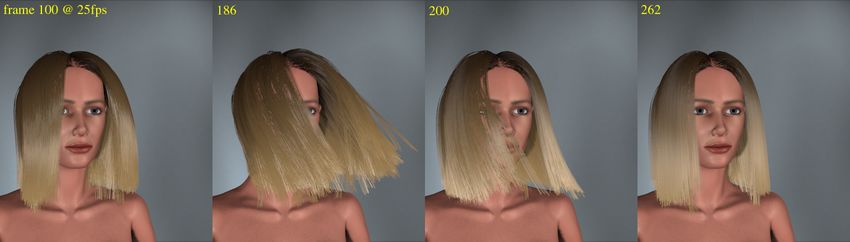
• The second animation scenario is to illustrate the "fluid" 7. Doo-Won Lee and Hyeong-Seok Ko. Natural
motion of hair without loosing the character of individual hairstyle modeling and animation. In Proceedings
hair. The hair volume starts falling freely under gravity. of International Workshop on Human Modeling and
Quickly, the individual hair’s length constraint and Animation, pages 11–21, Seoul, Korea, June 2000.
stiffness restricts the free falling motion to give it a Korea Computer Graphics Society. 1
bounce, towards end of the free fall (frame 53). At the
same time, "hair fluid" collides with the body and bursts 8. M. Lin and S. Gottschalk. Collision detection between
away sidewise (frame 70). The air interaction gives an geometric models: A survey. In Proceedings of IMA
overall damping. Observe that the hair quickly settles Conference on Mathematics of Surfaces, 1998. 2, 8
down, even after the sudden jerk in the motion, due to 9. Ronald L. Panton. Incompressible Flow. John Wiley,
air drag and hair friction with the body. 2nd edition edition, December 1995. 2, 3
• The third animation exclusively illustrates the
effectiveness of the model in animating hair blown 10. David Baraff. Linear-time dynamics using lagrange
by wind. Needless to say that there is an influence of multipliers. Proceedings of SIGGRAPH 96, pages 137–
airfield on individual hair. More importantly, body and 146, August 1996. 4
hair volume acts as a full and partial obstacle to air 11. Roy Featherstone. Robot Dynamics Algorithms.
altering its flow. Kluwer Academic Publishers, 1987. 4, 5
12. Brian Mirtich. Impulse-based Dynamic Simulation
8. Acknowledgements of Rigid Body Systems. PhD thesis, University of
California, Berkeley, December 1996. 5
This work is partially supported by Swiss National Research
Foundation (FNRS). Special thanks are due to Chris Joslin 13. Joseph Peter Morris. An overview of the method of
for proof reading this paper and to Prithweesh De for smoothed particle hydrodynamics. AGTM Preprints,
preparing the multimedia presentation. University of Kaiserslautern, 1995. 6, 7
14. Jos Stam. Stochastic dynamics: Simulating the
References effects of turbulence on flexible structures. Computer
Graphics Forum, 16(3):159–164, August 1997. 8
1. J.D. Gascuel, M.P. Cani, M. Desbrun, E. Leroy,
and C. Mirgon. Smoothed particles: A new 15. B. C. Vemuri, L. Chen, L. Vu-Quoc, X. Zhang, and
paradigm for animating highly deformable bodies. O. Walton. Efficient and accurate collision detection
In 6th Eurographics Workshop on Animation and for granular flow simulation. Graphical Models and
Simulation’96. Paris, September 1996. 1, 6 Image Processing, 60(5):403–422, November 1998. 8
c The Eurographics Association and Blackwell Publishers 2001.Sunil Hadap and Nadia Magnenat-Thalmann / Modeling Dynamic Hair as a Continuum
Figure 6: Approximate geometry, Smoothed particles, Octree
c The Eurographics Association and Blackwell Publishers 2001.You can also read