Modeling Image Patches with a Generic Dictionary of Mini-Epitomes
←
→
Page content transcription
If your browser does not render page correctly, please read the page content below
Modeling Image Patches with a Generic Dictionary of Mini-Epitomes

                George Papandreou                  Liang-Chieh Chen                   Alan L. Yuille
                  TTI Chicago                       UC Los Angeles                   UC Los Angeles
                  gpapan@ttic.edu                 lcchen@cs.ucla.edu              yuille@stat.ucla.edu

                         Abstract                                top of discriminative patch descriptors like SIFT [19]. SIFT
                                                                 has been explicitly designed for invariance to these nuisance
   The goal of this paper is to question the necessity of fea-   parameters, which allows it to work reliably in conjunction
tures like SIFT in categorical visual recognition tasks. As      with simple classification rules in a bag of visual words
an alternative, we develop a generative model for the raw        framework [17, 30]. However, the SIFT and other similar
intensity of image patches and show that it can support im-      descriptors are not suitable for image generation tasks and
age classification performance on par with optimized SIFT-       are very difficult to visualize [28].
based techniques in a bag-of-visual-words setting. Key in-           Instead of designing an image descriptor to be maxi-
gredient of the proposed model is a compact dictionary           mally invariant from the ground up, we attempt to explicitly
of mini-epitomes, learned in an unsupervised fashion on          model photometric and position nuisance parameters as at-
a large collection of images. The use of epitomes allows         tributes of a generative patch-based representation. Specifi-
us to explicitly account for photometric and position vari-      cally, we develop a probabilistic epitomic model which can
ability in image appearance. We show that this flexibility       faithfully reconstruct the raw appearance of an image patch
considerably increases the capacity of the dictionary to ac-     using just a single patch selected from a compact dictionary
curately approximate the appearance of image patches and         of mini-epitomes. Our first main contribution is to show
support recognition tasks. For image classification, we de-      that explicitly matching the image patches to their best po-
velop histogram-based image encoding methods tailored to         sition in the mini-epitomes greatly improves reconstruction
the epitomic representation, as well as an “epitomic foot-       accuracy compared to a non-epitomic baseline which does
print” encoding which is easy to visualize and highlights        not cater for position alignment. This allows us to accu-
the generative nature of our model. We discuss in detail         rately capture the appearance of image patches by a generic,
computational aspects and develop efficient algorithms to        i.e., universal rather than image specific, visual dictionary
make the model scalable to large tasks. The proposed tech-       learned from a large set of images.
niques are evaluated with experiments on the challenging
                                                                    We design image descriptors for image classification
PASCAL VOC 2007 image classification benchmark.
                                                                 tasks based on the proposed mini-epitomic dictionary. Our
                                                                 second main contribution is to show that bag-of-words type
                                                                 classifiers built on top of our epitomic representation not
1. Introduction                                                  only improve over ones built on non-epitomic patch dic-
   Our goal in this work is to investigate to which extent       tionaries, but also yield classification results competitive to
generative image models can also be competitive for visual       those based on the SIFT representation. Beyond histogram-
recognition tasks. We use the raw image patch intensity          type encodings, we also investigate an “epitomic footprint”
as the fundamental representation in our model. Appear-          encoding which captures how the appearance of a specific
ance patches have been successfully applied so far mostly        image deviates from the appearance of the generic dictio-
in image generation tasks such as texture synthesis, image       nary. This epitomic footprint descriptor can be visualized
denoising, and image super-resolution [2, 10, 12].               or stored as a small image and at the same time be used
   Using raw appearance patches maximally preserves in-          directly as feature vector in a linear SVM image classifier.
formation in the original image. The main challenge with            Employing the proposed model requires finding the best
this modeling approach in image classification tasks is that     match in the epitomic dictionary for each patch in an image.
the associated image description can be too sensitive to nui-    We have experimented with both a fast GPU implementa-
sance parameters such as illumination conditions or object       tion of exact search as well as approximate nearest neigh-
position. Therefore, most computer vision systems for im-        bor search techniques. Both allow efficient epitomic patch
age categorization and recognition rely on features built on     matching and image encoding in about 1 sec for 400×500
images and typical settings for the model parameter val-
ues, making the model scalable to large datasets. In the
main part of the paper we report image classification re-
sults on the challenging PASCAL VOC 2007 image clas-
sification benchmark [11] and compare the performance of
our model both with a non-epitomic baseline and the tuned
implementations of SIFT-based classification techniques re-
viewed by [6]. The supplementary material elaborates on
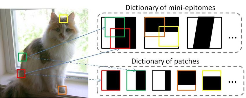
Figure 1. In the epitomic representation each image patch moves to
aspects of the proposed model and includes further experi-
find its best match within a mini-epitome. Search is over epitome
mental results on the Caltech-101 dataset. Accompanying positions instead of image positions (standard max-pooling).
software can be found at our web sites.
2. Related work 3. Image Modeling with Mini-Epitomes
Key element of the proposed method is the explicit mod- 3.1. Model description
eling of patch position using mini-epitomes. The epito-
With reference to Fig. 1, let {xi }Ni=1 be a set of possi-
mic image representation and the related idea of transfor-
bly overlapping image patches of size h × w pixels. Our
mation invariant clustering were developed in [13, 15] and
dictionary comprises K mini-epitomes {µk }K k=1 of size
also used in [31] for texture modeling, but have not been ap-
H × W , with H ≥ h and W ≥ w. The length of the
plied before for learning generic visual dictionaries on large
vectorized patches and epitomes is then d = h · w and
datasets and in the context of visual recognition tasks.
D = H·W , respectively. We approximate each image patch
The idea to use a patch-based representation for image
xi with its best match in the dictionary by searching over the
classification first appeared in [23] and was further devel-
Np = hp×wp (with hp = H − h + 1, wp = W − w + 1) dis-
oped by [26], who applied it to homogeneous texture classi-
tinct sub-patches of size h×w fully contained in each mini-
fication and compared it to the filterbank-based texton rep-
epitome. Typical sizes we employ are 8×8 for patches and
resentation of [18]. Recently, [7] demonstrated competi-
16×16 for mini-epitomes, implying that each mini-epitome
tive image classification results on the CIFAR-10 dataset of
can generate Np = 9 · 9 = 81 patches of size 8 × 8. Our
small images with patch dictionaries trained by K-means.
focus is on representing every image with a common vocab-
Neither of these works explicitly handles patch position or
ulary of visual words, so we use a single universal epitomic
demonstrates performance comparable to modern SIFT en-
dictionary for analyzing image patches from any image. We
codings [6] on challenging large-scale classification tasks.
have been working with datasets consisting of overlapping
More generally, unsupervised learning of image features
patches extracted from thousands of images and with dictio-
has received considerable attention recently. Most related
naries containing from K = 32 up to 2048 mini-epitomes.
to our work is [29], which also attempts to explicitly model
We model the appearance of image patches using a Gaus-
the position of visual patterns in a deconvolutional model.
sian mixture model (GMM). We employ a generative model
However, their model requires iteratively solving a large-
in which we activate one of the image epitomes µk with
scale sparse coding problem both during train and test time.
probability P (li = k) = πk , then crop an h×w sub-patch
The image classification performance they report signifi-
from it by selecting the position pi = (xi , yi ) of its top-
cantly lags modern SIFT-based models such as those de-
left corner uniformly at random from any of the Np valid
scribed in [6], despite the fact that they learn a multi-layered
positions. We assume that an image patch xi is then condi-
feature representation. The power of learned patch-level
tionally generated from a multivariate Gaussian distribution
features has also been demonstrated recently in [5, 9, 24].
Using mini-epitomes instead of image patches could also P (xi |zi , θ) = N (xi ; αi Tpi µli + βi 1, c2i Σ0 ) . (1)
prove beneficial in their setting.
Sparsity provides a compelling framework for learning The label/position latent variable vector zi = (li , xi , yi )
image patch dictionaries [22]. Sparsity coupled with epit- controls the Gaussian mean via νzi = Tpi µli . Here
omes has been explored in [1, 4] but these works focus on Tpi is a d × D projection matrix of zeros and ones which
learning dictionaries on a single or a few images. While crops the sub-patch at position pi = (xi , yi ) of a mini-
each image patch is represented as a linear combination of epitome. The scalars αi and βi determine an affine map-
a few dictionary elements in sparse models, it is approxi- ping on the appearance vector and account for some pho-
mated by just one dictionary element in our model. One tometric variability, 1 is the all-ones d × 1 vector, and x̄
can thus think of the proposed model as an extremely sparse is the patch mean value. In the experiments reported in
representation, or alternatively as an epitomic form of K- this paper we choose πk = 1/K and fix the d × d covari-
means or vector quantization. ance matrix Σ−10 = DT D + ǫI, where D is the gradi-ent operator computing the x− and y− derivatives of the 3.3. Efficient epitomic search algorithms
h×w patch and ǫ is a small constant. This implies that we
We search over all mini-epitomes and positions in them
compute distances between patches by a Mahalanobis met-
to select the mini-epitome label and position pair (k, p)
ric which corresponds to whitening the vectorized image
which achieves the least reconstruction error. The most ex-
patches by left-multiplying them with D. Importantly, we
pensive part of this matching process is computing the inner
assume that Σ0 is modulated by the patch gradient contrast
product of every patch in an image with all h×w sub-patches
c2i , kD(xi − x̄i 1)k22 + λ but is shared across all dictionary
in every mini-epitome in the dictionary.
elements and thus does not depend on the latent variable
vector; λ is a small regularization constant (we use λ = d
for image values between 0 and 255). We present algo- Exact search The complexity of the straightforward algo-
rithms for learning the epitomic means {µk }K k=1 in Sec. 3.4. rithm for matching N image patches to a dictionary with K
mini-epitomes is O(N · K · hp · wp · h · w). For the patch and
3.2. Epitomic patch matching epitome sizes we explore in our experiments, it takes more
than 10 sec to exactly match a 400 × 500 grayscale image
To match a patch xi to the dictionary, we seek the mini- with an optimized Matlab CPU implementation. Our opti-
epitome label and position zi = (li , xi , yi ), as well as mized GPU software has drastically reduced this computa-
the photometric correction parameters (αi , βi ) that maxi- tion time: for a dictionary with K=256 mini-epitomes, epit-
mize the probability in Eq. (1), or equivalently minimize omic matching takes 0.7 sec on a laptop’s NVIDIA GTX
the squared reconstruction error (note that D1 = 0) 650M graphics unit and 0.1 sec on a workstation’s NVIDIA
Tesla K20. The starting point of our implementation has
1 been the fast CUDA convolution library cuda-convnet [16]
R2 (xi ; k, p) = 2 kD (xi − αi Tp µk )k2 + λ(|αi | − 1)2 , but we are able to achieve epitome-specific improvements
ci
(2) by exploiting the fact that patches within a mini-epitome
where the last regularization term discourages matches be- share filter values, which allows us to make better use of
tween patches and mini-epitomes whose contrast widely the GPU’s fast shared memory. As a result, matching with
differs. We can compute in closed form for each candi- a 16 × 16/8 × 8 epitomic dictionary is only about 5 times
date match νzi = Tpi µli in the dictionary the optimal more expensive than matching with a non-epitomic 8×8 dic-
x̃T ν̃ ±λ tionary, although the epitomic dictionary contains 81 times
β̂i = x̄i − α̂i ν̄zi and α̂i = ν̃ Ti ν̃zzi +λ , where x̃i = Dxi more patches. We have also tested the recursive algorithm
zi i
and ν̃zi = Dνzi are the whitened patches. The sign in of [21] and FFT techniques [13], but they have proven less
the nominator is positive if x̃Ti ν̃zi ≥ 0 and negative oth- efficient than our GPU code for the range of epitome and
erwise. Having computed the best photometric correction patch sizes we have experimented with.
parameters, we can substitute back in Eq. (2) and evaluate
the reconstruction error R2 (xi ; k, p).
Approximate search We have also investigated the use
of approximate nearest neighbor (ANN) methods for epit-
omic patch matching. Contrary to exact search methods,
Epitomic matching versus max-pooling Searching for ANN search time typically grows sub-linearly with the dic-
the best match in the epitome resembles the max-pooling tionary size, and is thus better scalable to extremely large
process in convolutional neural networks [14]. However in dictionary sizes. The approach we have followed is to ex-
these two models the roles of dictionary elements and im- tract all patches from each mini-epitome along with their
age patches are reversed: In epitomic matching, each im- negated pairs, whiten, and then normalize them to be unit-
age patch is assigned to one dictionary element. On the norm vectors, resulting in an inflated epitomic dictionary
other hand, in max-pooling each dictionary element (fil- with K · Np · 2 elements. After similarly whitening and
ter in the terminology of [14]) looks for its best matching normalizing the input image patches, we search for their
patch within a search window. Max-pooling thus typically best match with standard off-the-shelf kd-tree and hierar-
assigns some image patches to multiple filters while other chical kmeans algorithms as implemented in the FLANN
patches may remain orphan. This subtle but crucial differ- library [20]. When using kd-trees, we have found it crucial
ence makes it difficult for max-pooling to be used as a basis to apply a rotation transformation based on the fast 2-D dis-
for building whole image probabilistic models, as the prob- crete cosine transform (DCT), instead of searching directly
ability of orphan image areas is not well defined. Contrary for the best match in the image gradient domain. We pro-
to that, mini-epitomes naturally lend themselves as building vide more details about this important technical point in the
blocks for probabilistic image models able to explain and supplementary material. We also present experiments there
generate the whole image area. which show that the performance loss due to ANN is neg-(a) Our epitomic patch dictionary (K = 256) (b) Non-epitomic dictionary (K = 1024)
Figure 2. Patch dictionaries learned on the full VOC 2007 training set, ordered column-wise from top-left by their relative frequency.
ligible, for moderate search times comparable to those of Diverse dictionary initialization with epitomic K-
SIFT-based VQ encoding algorithms. means++ Careful parameter initialization helps EM con-
verge faster and reach a good local optimum solution. The
3.4. Epitomic dictionary learning K-means++ algorithm [3] selects a diverse subset of train-
Parameter refinement by Expectation-Maximization ing data instances as initialization to dictionary learning. It
Given a large training set of unlabeled image patches randomly picks the first one and then incrementally grows
{xi }N
i=1 , our goal is to learn the maximum likelihood model
the dictionary by selecting subsequent elements with proba-
parameters θ = {µk }K k=1 ) for the epitomic GMM model in
bility proportional to their squared distance to the elements
Eq. (1). We employ the EM algorithm [8] and maximize the already in the dictionary. We adapt the standard K-means++
expected complete log-likelihood algorithm to our epitomic setup and select a H×W training
image patch as a new mini-epitome with probability propor-
N X
X K X tional to the sum of R2 (xi ; k, p) in a neighborhood of size
L(θ) = γi (k, p)· hp ×wp around the i-th patch. This corresponds to spatially
i=1 k=1 p∈P smoothing the squared reconstruction error R2 (xi ; k, p) by
a hp ×wp box filter.
log πk N (xi ; αi Tp µk + βi 1, c2i Σ0 ) , (3)
where P is the set of valid positions in the epitome. In the
Learned epitomic dictionary We show in Fig. 2 the epit-
E-step, we compute the assignment of each patch to the dic-
omic dictionary with K = 256 mini-epitomes we learned
tionary, given the current model parameter values. We use
with the proposed algorithm on the full VOC 2007 training
the hard assignment version of EM and set γi (k, p) = 1 if
set. We juxtapose it with the corresponding non-epitomic
the i-th patch best matches in the p-th position in the k-th
dictionary with K = 1024 members we learned with the
mini-epitome and 0 otherwise. In the M-step, we update
same algorithm, simply setting H = W = h = w = 8. We
each of the K mini-epitomes µk by
have chosen the non-epitomic dictionary to have 4 times
as many members so as both dictionaries occupy the same
αi2 T −1
X
γi (k, p) T Σ T p µk = area (note that 162 /82 = 4) and thus be commensurate in
i,p
c2i p 0 the sense that they have equal number of parameters.
X αi As expected, the non-epitomic dictionary looks very
γi (k, p) 2 TTp Σ−1
0 (xi − βi 1) . (4)
i,p
ci similar to the K-means patch dictionaries reported in [7].
Our epitomic dictionary looks qualitatively different: It
In all reported experiments we run EM for 10 iterations. is more diverse and contains a rich set of visual pat-We can also reconstruct the original full-sized images by
placing the reconstructed patches x̂i in their corresponding
image positions and averaging at each pixel the values of
all overlapping patches that contain it. We quantify the full
image reconstruction quality in terms of PSNR. We show
an example of such an image reconstruction in Fig. 3(a,b).
Note that reconstructing an image from its SIFT descriptor
[28] is far less accurate and less straightforward than using
a generative image model such as the proposed one.
To evaluate the reconstruction ability of each dictionary,
we plot in Fig. 4 the empirical complementary cumulative
distribution function (CCDF=1-CDF, where CDF is the cu-
(a) Original image (b) Reconstructed (PSNR=29.2dB) mulative distribution function) for the selected metrics. If
55
Image Reconstruction PSNR Scatterplot
450
Image Reconstruction PSNR Difference
p = CCDF(v), then p×100% of the samples in the dataset
50 400 have values at least equal to v (higher CCDF curves are bet-
350
PSNR (Epitome)
45
300 ter). The plots summarize VOC 2007 test set statistics of:
40 250
200
(a/b) the NCC/ NCCD for all N ≈ 5×10⁷ patches and (c)
35
30
150 the PSNR for all 4952 images.
100
25 50
There are several observations we can make by inspect-
20
20 25 30 35 40 45 50
0
−0.5 0 0.5 1 1.5 2 2.5 3 ing Fig. 4. First, for either dictionary type, whenever we
PSNR (NonEpitome) PSNR (Epitome) − PSNR (NonEpitome)
double the dictionary size K, the CCDF curves shift to the
(c) Epitome vs. Non-epitome PSNR right/up by a rouphly constant step. For example, we can
Figure 3. (a,b) Image reconstruction example with the K = 512
read from Fig. 4(a) that the K = 32 epitomic dictionary
epitomic dictionary. (c) Image reconstruction on VOC 2007 test
already suffices to explain 58% of the image patches with
set: K = 512 epitomic vs. K = 2048 non-epitomic dictionaries.
NCC ≥ 0.8. Each time we double K we explain 3% more
image patches at this level, with the K = 512 epitomic dic-
terns, including sharp edges, lines, corners, junctions, and tionary being able to reconstruct 70% of the image patches
sinewaves. It has less spatial redundancy than its non- at NCC ≥ 0.8. In comparison, the K = 2048 non-epitomic
epitomic counterpart, which needs to encode shifted ver- baseline can only reconstruct 62% of the image patches at
sions of the same pattern as distinct codewords. the same accuracy level.
Second, comparing the performance of the two dictio-
3.5. Reconstructing patches and images nary types, we observe that our epitomic model signifi-
Beyond qualitative comparisons, we have tried to sys- cantly improves over the non-epitomic baseline in terms
tematically evaluate the generative expressive power of our of reconstruction accuracy. For example, we can see that
epitomic dictionary compared to the non-epitomic baseline. the K = 64 epitomic dictionary is roughly as accurate
as the K = 2048 non-epitomic dictionary which has 32
For this purpose, having trained the two dictionaries on
times more elements (the same holds for the K = 32/1024
the PASCAL VOC 2007 train set, we have quantified how
dictionaries). Accounting for the fact that each 16 × 16
accurately they perform in reconstructing the images in the
mini-epitome occupies 4 times larger area than each clus-
full VOC 2007 test set. From each test image, we ex-
ter center of the 8×8 non-epitomic dictionary, implies that
tract its 8 × 8 overlapping patches (with stride 2 pixels in
the epitomic dictionary is 32/4 = 8 times more compact
each direction) that form the set of ground truth patches
(in terms of number of model parameters) than the non-
{xi }N
i=1 . For each patch xi we compute its closest match
epitomic baseline. We further show in Fig. 3(c) that the
x̂i = (αi Tp µk + βi 1) in each of the two dictionaries by
epitomic dictionary consistently performs better (except for
finding the parameters (αi , βi ) and (k, p) that minimize the
1 out of the 4952 test images) in terms of image reconstruc-
squared reconstruction R2 (xi ; k, p) in Eq. (2) – note that
tion PSNR (1.34 dB on average).
p = (0, 0) in the non-epitomic case.
We quantify how close xi and x̂i are in terms of nor-
malized cross-correlation in both the raw intensity and 4. Image Classification with Mini-Epitomes
T
gradient domains, NCC(i) = (x i −x̄i ) (x̂i −x̄i )+λ
kxi −x̄i kλ kx̂i −x̄i kλ and 4.1. Image classification tasks
(xi −x̄i )T DT D(x̂i −x̄i )+λ
NCCD (i) = kD(xi −x̄i )kλ kD(x̂i −x̄i )kλ respectively, where Here we show how the proposed dictionary of mini-
T 1/2
kxkλ , (x x + λ) . Note that NCC takes values be- epitomes can be used in image classification tasks. We fo-
tween 0 (poor match) and 1 (perfect match). cus our evaluation on the challenging PASCAL VOC 20071 1 1
0.9 0.9 0.9
← K=512 ← K=512 ← K=512
0.8 0.8 0.8
K=2048→ K=2048→ K=2048→
0.7 0.7 0.7
← K=32 ← K=32 ← K=32
1 − CDF
0.6 0.6 0.6
K=128→ K=128→ K=128→
0.5 0.5 0.5
0.4 0.4 0.4
0.3 0.3 0.3
0.2 NonEpitome 0.2 0.2
0.1 Epitome 0.1 0.1
0 0 0
0.3 0.4 0.5 0.6 0.7 0.8 0.9 10.3 0.4 0.5 0.6 0.7 0.8 0.9 1 22 24 26 28 30 32 34 36 38 40
Normalized Cross−Correlation Normalized Cross−Correlation PSNR (dB)
(a) Raw image patches (b) Whitened image patches (c) Whole images
Figure 4. Image reconstruction evaluation on the full VOC 2007 test set with our epitomic patch dictionary vs. a non-epitomic dictionary
for various dictionary sizes K (powers of 2). (a,b): Normalized cross-correlation of raw (NCC) and whitened (NCCD ) image patches.
(c): PSNR of reconstructed whole images. Plots depict 1-CDF (higher is better).
image classification benchmark [11]. total length K · t · t. For example, in the Epitome-16/8-Pos-
We extract histogram-type features from both epitomic 4x4 descriptor the epitomic position bins have size 3 × 3
and non-epitomic patch representations which we feed to pixels and stride 2 pixels in each direction. The (bx , by ) bin
1-vs-all SVM classifiers. We use χ2 kernels approximated (bx , by = 0 : 3) gets a vote for each matched patch whose
by explicit feature maps [27] and also employ spatial pyra- position pi = (xi , yi ) satisfies 2bx ≤ xi < 2bx + 3 and
mid matching [17]. Our implementation closely follows the 2by ≤ yi < 2by + 3.
publicly available setup of [6], which presents a systematic In all experiments we also encode the sign of the match,
evaluation and tuned implementation of SIFT features cou- putting matches with positive and negative αi ’s in different
pled with state-of-the-art encoding techniques. bins, which we have found to considerably improve perfor-
mance at the cost of doubling the descriptor size.
4.2. Image description with mini-epitomes
4.3. Classification results
Here we focus on extracting histogram type descriptors
treating our epitomic dictionary as a bag of visual words. For all the results involving the epitomic as well as the
From each image, we densely extract h × w overlapping non-epitomic patch models, we have learned dictionaries of
patches {xi }N i=1 (with stride 2 pixels in each direction). various sizes on the full VOC 2007 train set. We summarize
Matching each patch xi to the epitomic dictionary yields its our results in Table 1 and illustrate them with plots in Fig. 5.
closest h×w patch in the epitomic dictionary, encoded by We first explore in Fig. 5(a) how epitome and patch sizes
the epitomic label li ∈ 1 : K and the position pi = (xi , yi ), as well as dictionary sizes affect the performance of the epit-
with xi = 0 : wp − 1 and yi = 0 : hp − 1. We use hard omic model. We find that the performance of the epitomic
assignments (VQ) in all reported results. model is not too sensitive to the exact setting of the epit-
In this setting, the most straightforward way to summa- ome/patch size. Similarly to the findings of [7], we observe
rize the content of an image is to build a histogram with K that the performance of all descriptors increases when we
bins, each counting how many times the specific epitome use dictionaries with more elements.
has been activated. This “Epitome-Pos-1x1 ” descriptor is In Fig. 5(b) we show that position encoding considerably
very compact but completely discards the exact position of improves the recognition performance of the epitomic dic-
the match within the epitome. tionary, with the coarse 2×2 scheme exhibiting an excellent
Our epitomic dictionary allows us to also encode the po- trade-off between performance and descriptor size.
sition information pi into the descriptor. While some of the We can evaluate the proposed epitomic model relative
H ×W mini-epitomes in our learned dictionary (see Fig. 2) to the non-epitomic baseline along multiple axes. First, as
are homogeneous, others contain h × w patches with visu- we can see in Figs. 5(a,b), the epitomic dictionary performs
ally diverse appearance. We can encode the exact position much better than the non-epitomic baseline for fixed dic-
pi of the match in the epitome by a product histogram with tionary size K. Second, we can see in Fig. 5(c) that epit-
K · Np bins, where Np = hp ×wp . However this yields a omes have an edge over non-epitomes for fixed histogram
rather large descriptor (note that Np = 81 in our setting) descriptor length K · t · t. Note that descriptor length di-
which is very sensitive to the exact position. We opt instead rectly affects the classifier training and evaluation time, as
to encode the epitome position pi more coarsely. Specifi- well as the number of labeled data required for training.
cally, we summarize the match positions in a t × t spatial Third, epitomes perform better than non-epitomes when
grid of bins yielding an “Epitome-Pos-t×t” descriptor with the two models have the same number of parameters, e.g.,Epitome Position Dictionary Size K Method mAP Method mAP Method mAP
/Patch Encod. 32 64 128 256 512 1024 2048 VQ-4K 53.42 KCB-4K 54.60 LLC-4K 53.79
16/8 1x1 40.66 45.22 48.07 49.00 51.98 53.54 54.37 VQ-10K 54.98 KCB-25K 56.26 LLC-10K 56.01
2x2 47.11 49.89 51.59 52.89 54.50 56.12 56.16 VQ-25K 56.07 FV-256 61.69 LLC-25K 57.60
4x4 49.59 51.98 53.10 54.75 55.62 56.45 56.18 Table 2. Image classification results (mAP) of top-performing
9x9 52.03 53.53 54.03 54.07 - - - SIFT-based methods on the Pascal VOC 2007 dataset [6].
12/8 1x1 41.01 44.94 47.24 49.56 51.76 53.48 55.33
2x2 46.20 47.89 50.19 51.91 53.64 55.17 56.47
10/8 1x1 41.12 44.07 46.85 49.33 51.28 53.01 54.87
2x2 44.10 46.32 48.71 50.98 52.85 54.52 55.71 vector Fisher Vector encoding in [25]. The main idea is to
2x2/4 44.46 46.73 48.37 51.03 52.31 54.33 55.08 encode the difference between the appearance content of a
12/6 1x1 40.69 43.83 46.55 49.73 51.05 52.37 54.24
2x2 46.80 48.72 50.96 52.70 53.91 54.80 55.40
specific image compared to the generic epitome, which cap-
3x3 48.43 50.40 52.17 53.45 55.16 55.11 55.47 tures how much the epitome needs to adapt to best approxi-
8/8 1x1 38.02 40.92 44.54 46.75 48.84 51.13 52.73 mate a novel image. An appealling property of the epitomic
6/6 1x1 38.17 41.89 45.01 47.35 48.88 51.15 52.85 footprint descriptor is that it can be visualized or stored as
Table 1. Image classification results (mAP) of our epitomic dictio- a small image and at the same time be used directly as fea-
nary on the Pascal VOC 2007 dataset. ture vector in a linear SVM image classifier, yielding per-
formance around 52% mAP in our experiments. Please see
Fig.6 for a visualization and the supplementary material for
further details and examples.
the K = 512 Epitome-16/8-Pos-2x2 dictionary achieves
54.50 mAP vs. 52.73 mAP of the comparable K = 2048
Non-Epitome-8/8. Fourth, we compare epitomes and non-
epitomes that require the same number of reconstruction
error computations for matching with the exact search al-
gorithm (note however that Sec. 3.3 presents more efficient
matching algorithms for epitomes). For this purpose, we
run an experiment with the K element Epitome-10/8-Pos-
2x2 dictionary and only searching at 4 candidate positions
(xi , yi ) ∈ {0, 2}2 in each mini-epitome (2x2/4 entry in Ta- (a) Image (b) Epitomic footprint
ble 1 and Fig. 5(c)). This performs very similarly to the Figure 6. Epitomic footprint descriptor.
comparable 4 · K element Non-Epitome-8/8 dictionary.
Overall, classification performance of both models is
strongly correlated with the total number of patches con- 5. Discussion and Future Work
tained in the dictionary, yet the epitomic representation
offers distinct advantages over the non-epitomic baseline: We have shown that explicitly accounting for illumina-
It generates a given number of patches with much fewer tion and position variability can significantly improve both
model parameters, it controls the descriptor length by ad- reconstruction and classification performance of a patch-
justing the coarseness of epitome position encoding, and is based image dictionary. Moreover, we have demonstrated
amenable to fast search. that the proposed epitomic model can perform similarly to
Comparing with the performance of VQ descriptors SIFT in image classification, implying that generative patch
based on SIFT, see Table 2, the most impressive finding is image models can be competitive with discriminative de-
that epitomic descriptors built on dictionaries with as few as scriptors when properly accounting for nuisance factors.
K = 256 or 512 mini-epitomes yield performance around In future work, we plan to extend the current system to-
55% mAP, which takes SIFT dictionaries of size 10K to wards capturing visual attributes such as depth or color and
achieve. Our best result at 56.47% mAP with 2048 mini- modeling a richer set of spatial transformations, including
epitomes even slightly outperforms the best SIFT VQ re- scale and rotation. We also plan to build deep variants of
sult reported in [6], attained with a dictionary of 25K visual our model, employing epitomes in hierarchical models.
words. This result is also comparable to KCB and LLC-
based methods for encoding SIFT but still lags behind the
state-of-the-art Fisher Vector descriptor whose performance Acknowledgments
is about 61% mAP [6, 25]. This work was supported by the ONR grant N00014-10-1-
0933 and by the NIH grant 5R01EY022247-03. We would
Epitomic footprint encoding We have also explored an like to thank Prof. T.-S. Lee and the anonymous reviewers
epitomic footprint encoding, which is related to the mean- for their extensive feedback on this paper.VOC 2007 Classification Results VOC 2007 Classification Results VOC 2007 Classification Results
60 60 60
55 55 55
50 50 50
mAP (%)
mAP (%)
mAP (%)
45 45 45
Epitome 16/8 (Pos−1x1)
Epitome 12/8 (Pos−1x1) Epitome 16/8 (Pos−9x9) Epitome 16/8 (Pos−2x2)
Epitome 10/8 (Pos−1x1) Epitome 16/8 (Pos−4x4) Epitome 12/8 (Pos−2x2)
40 Epitome 12/6 (Pos−1x1) 40 Epitome 16/8 (Pos−2x2) 40 Epitome 10/8 (Pos−2x2)
Non−Epitome 8/8 Epitome 16/8 (Pos−1x1) Epitome 10/8 (Pos−2x2/4)
Non−Epitome 6/6 Non−Epitome 8/8 Non−Epitome 8/8
35 35 35
32 64 128 256 512 1024 2048 32 64 128 256 512 1024 2048 128 256 512 1024 2048 4096 8192
Dictionary size Dictionary size Total histogram size (LabelxPosition)
(a) (b) (c)
Figure 5. (a) Performance of the epitomic dictionary model (without epitome position encoding) and the non-epitomic baseline for different
epitome/patch sizes, as a function of dictionary size K. (b) Effect of encoding the epitome position at different detail levels. (c) Comparison
of the epitomic model (with or without position encoding) and the non-epitomic baseline, for the same total histogram length.
References [16] A. Krizhevsky, I. Sutskever, and G. Hinton. ImageNet clas-
sification with deep convolutional neural networks. In NIPS,
[1] M. Aharon and M. Elad. Sparse and redundant modeling of 2013.
image content using an image-signature-dictionary. SIAM J. [17] Z. Lazebnik, C. Schmid, and J. Ponce. Beyond bags of
Imaging Sci., 1(3):228–247, 2008. features: Spatial pyramid matching for recognizing natural
[2] M. Aharon, M. Elad, and A. Bruckstein. K-SVD: An al- scene categories. In CVPR, 2006.
gorithm for designing overcomplete dictionaries for sparse [18] T. Leung and J. Malik. Representing and recognizing the
representation. IEEE Trans. Signal Process., 54(11):4311– visual appearance of materials using three-dimensional tex-
4322, 2006. tons. IJCV, 43(1):29–44, 2001.
[3] D. Arthur and S. Vassilvitskii. K-means++: The advantages [19] D. Lowe. Distinctive image features from scale-invariant
of careful seeding. In Proc. SODA, 2007. keypoints. IJCV, 60(2):91–110, 2004.
[4] L. Benoı̂t, J. Mairal, F. Bach, and J. Ponce. Sparse image [20] M. Muja and D. Lowe. Fast approximate nearest neighbors
representation with epitomes. In CVPR, 2011. with automatic algorithm configuration. In VISAPP, 2009.
[5] L. Bo, X. Ren, and D. Fox. Hierarchical matching pursuit [21] I. Olonetsky and S. Avidan. Treecann - k-d tree coherence
for image classification. In NIPS, 2011. approximate nearest neighbor algorithm. In ECCV, 2012.
[6] K. Chatfield, V. Lempitsky, A. Vedaldi, and A. Zisserman. [22] B. Olshausen and D. Field. Emergence of simple-cell re-
The devil is in the details: an evaluation of recent feature ceptive field properties by learning a sparse code for natural
encoding methods. In BMVC, 2011. images. Nature, 381:607–609, 1996.
[7] A. Coates, H. Lee, and A. Ng. An analysis of single-layer [23] K. Popat and R. Picard. Cluster-based probability model and
networks in unsupervised feature learning. In AISTATS, its application to image and texture processing. IEEE Trans.
2011. Image Process., 6(2):268–284, 1997.
[8] A. P. Dempster, N. M. Laird, and D. B. Rubin. Maxi- [24] X. Ren and D. Ramanan. Histograms of sparse codes for
mum Likelihood from incomplete data via the EM algorithm. object detection. In CVPR, 2013.
JRSS (B), 39(1):1–38, 1977. [25] J. Sánchez, F. Perronnin, T. Mensink, and J. J. Verbeek. Im-
[9] M. Dikmen, D. Hoiem, and T. Huang. A data driven method age classification with the Fisher vector: Theory and prac-
for feature transformation. In CVPR, 2012. tice. IJCV, 105(3):222–245, 2013.
[10] A. Efros and W. Freeman. Image quilting for texture synthe- [26] M. Varma and A. Zisserman. A statistical approach to tex-
sis and transfer. In SIGGRAPH, 2001. ture classification from single images. IJCV, 62(1-2):61–81,
[11] M. Everingham, L. Van Gool, C. Williams, J. Winn, and 2005.
A. Zisserman. The PASCAL visual object classes challenge. [27] A. Vedaldi and A. Zisserman. Efficient additive kernels via
IJCV, 88(2):303–338, 2010. explicit feature maps. PAMI, 34(3):480–492, 2012.
[12] W. Freeman, E. Pasztor, and O. Carmichael. Learning low- [28] P. Weinzaepfel, H. Jégou, and P. Pérez. Reconstructing an
level vision. IJCV, 40(1):25–47, 2000. image from its local descriptors. In CVPR, 2011.
[13] B. Frey and N. Jojic. Transformation-invariant clustering us- [29] M. Zeiler, D. Krishnan, G. Taylor, and R. Fergus. Deconvo-
ing the EM algorithm. PAMI, 25(1):1–17, 2003. lutional networks. In CVPR, 2010.
[14] K. Jarrett, K. Kavukcuoglu, M. Ranzato, and Y. LeCun. [30] J. Zhang, M. Marszalek, S. Lazebnik, and C. Schmid. Local
What is the best multi-stage architecture for object recog- features and kernels for classification of texture and object
nition? In ICCV, 2009. categories. IJCV, 73(2):213–238, 2007.
[31] S. Zhu, C. Guo, Y. Wang, and Z. Xu. What are textons?
[15] N. Jojic, B. Frey, and A. Kannan. Epitomic analysis of ap-
IJCV, 62(1-2):121–143, 2005.
pearance and shape. In ICCV, 2003.You can also read