Modeling the World from Internet Photo Collections
←
→
Page content transcription
If your browser does not render page correctly, please read the page content below
Int J Comput Vis
DOI 10.1007/s11263-007-0107-3

Modeling the World from Internet Photo Collections
Noah Snavely · Steven M. Seitz · Richard Szeliski

Received: 30 January 2007 / Accepted: 31 October 2007
© Springer Science+Business Media, LLC 2007

Abstract There are billions of photographs on the Inter-        and changes in season, weather, and decade. Furthermore,
net, comprising the largest and most diverse photo collec-      entire cities are now being captured at street level and from
tion ever assembled. How can computer vision researchers        a birds-eye perspective (e.g., Windows Live Local,1,2 and
exploit this imagery? This paper explores this question from    Google Streetview3 ), and from satellite or aerial views (e.g.,
the standpoint of 3D scene modeling and visualization. We       Google4 ).
present structure-from-motion and image-based rendering             The availability of such rich imagery of large parts of
algorithms that operate on hundreds of images downloaded        the earth’s surface under many different viewing conditions
as a result of keyword-based image search queries like          presents enormous opportunities, both in computer vision
“Notre Dame” or “Trevi Fountain.” This approach, which          research and for practical applications. From the standpoint
we call Photo Tourism, has enabled reconstructions of nu-       of shape modeling research, Internet imagery presents the
merous well-known world sites. This paper presents these        ultimate data set, which should enable modeling a signifi-
algorithms and results as a first step towards 3D modeling of   cant portion of the world’s surface geometry at high resolu-
the world’s well-photographed sites, cities, and landscapes     tion. As the largest, most diverse set of images ever assem-
from Internet imagery, and discusses key open problems and      bled, Internet imagery provides deep insights into the space
challenges for the research community.                          of natural images and a rich source of statistics and priors for
                                                                modeling scene appearance. Furthermore, Internet imagery
Keywords Structure from motion · 3D scene analysis ·            provides an ideal test bed for developing robust and gen-
Internet imagery · Photo browsers · 3D navigation               eral computer vision algorithms that can work effectively
                                                                “in the wild.” In turn, algorithms that operate effectively on
                                                                such imagery will enable a host of important applications,
1 Introduction                                                  ranging from 3D visualization, localization, communication
                                                                (media sharing), and recognition, that go well beyond tradi-
Most of the world’s significant sites have been photographed    tional computer vision problems and can have broad impacts
under many different conditions, both from the ground and       for the population at large.
from the air. For example, a Google image search for “Notre         To date, this imagery is almost completely untapped and
Dame” returns over one million hits (as of September,           unexploited by computer vision researchers. A major rea-
2007), showing the cathedral from almost every conceivable      son is that the imagery is not in a form that is amenable to
viewing position and angle, different times of day and night,   processing, at least by traditional methods: the images are

N. Snavely () · S.M. Seitz                                     1 Windows   Live Local, http://local.live.com.
University of Washington, Seattle, WA, USA                      2 Windows  Live Local—Virtual Earth Technology Preview, http://
e-mail: snavely@cs.washington.edu                               preview.local.live.com.
                                                                3 Google   Maps, http://maps.google.com.
R. Szeliski
                                                                4 Google   Maps, http://maps.google.com.
Microsoft Research, Redmond, WA, USA
Int J Comput Vis

unorganized, uncalibrated, with widely variable and uncon-      keypoints at a single scale, modern techniques use a quasi-
trolled illumination, resolution, and image quality. Develop-   continuous sampling of scale space to detect points invari-
ing computer vision techniques that can operate effectively     ant to changes in scale and orientation (Lowe 2004; Mikola-
with such imagery has been a major challenge for the re-        jczyk and Schmid 2004) and somewhat invariant to affine
search community. Within this scope, one key challenge is       transformations (Baumberg 2000; Kadir and Brady 2001;
registration, i.e., figuring out correspondences between im-    Schaffalitzky and Zisserman 2002; Mikolajczyk et al. 2005).
ages, and how they relate to one another in a common 3D             Unfortunately, early techniques relied on matching
coordinate system (structure from motion). While a lot of       patches around the detected keypoints, which limited their
progress has been made in these areas in the last two decades   range of applicability to scenes seen from similar view-
(Sect. 2), many challenging open problems remain.               points, e.g., for aerial photogrammetry applications (Hannah
    In this paper we focus on the problem of geometrically      1988). If features are being tracked from frame to frame, an
registering Internet imagery and a number of applications       affine extension of the basic Lucas-Kanade tracker has been
that this enables. As such, we first review the state of the    shown to perform well (Shi and Tomasi 1994). However, for
art and then present some first steps towards solving this      true wide baseline matching, i.e., the automatic matching of
problem along with a visualization front-end that we call       images taken from widely different views (Baumberg 2000;
Photo Tourism (Snavely et al. 2006). We then present a set      Schaffalitzky and Zisserman 2002; Strecha et al. 2003;
of open research problems for the field, including the cre-     Tuytelaars and Van Gool 2004; Matas et al. 2004), (weakly)
                                                                affine-invariant feature descriptors must be used.
ation of more efficient correspondence and reconstruction
                                                                    Mikolajczyk et al. (2005) review some recently devel-
techniques for extremely large image data sets. This paper
                                                                oped view-invariant local image descriptors and experimen-
expands on the work originally presented in (Snavely et al.
                                                                tally compare their performance. In our own Photo Tourism
2006) with many new reconstructions and visualizations of
                                                                research, we have been using Lowe’s Scale Invariant Fea-
algorithm behavior across datasets, as well as a brief dis-
                                                                ture Transform (SIFT) (Lowe 2004), which is widely used
cussion of Photosynth, a Technology Preview by Microsoft
                                                                by others and is known to perform well over a reasonable
Live Labs, based largely on (Snavely et al. 2006). We also
                                                                range of viewpoint variation.
present a more complete related work section and add a
broad discussion of open research challenges for the field.     2.2 Structure from Motion
Videos of our system, along with additional supplementary
material, can be found on our Photo Tourism project Web         The late 1980s also saw the development of effective struc-
site, http://phototour.cs.washington.edu.                       ture from motion techniques, which aim to simultaneously
                                                                reconstruct the unknown 3D scene structure and camera
                                                                positions and orientations from a set of feature correspon-
2 Previous Work                                                 dences. While Longuet-Higgins (1981) introduced a still
                                                                widely used two-frame relative orientation technique in
The last two decades have seen a dramatic increase in the       1981, the development of multi-frame structure from mo-
capabilities of 3D computer vision algorithms. These in-        tion techniques, including factorization methods (Tomasi
clude advances in feature correspondence, structure from        and Kanade 1992) and global optimization techniques (Spet-
                                                                sakis and Aloimonos 1991; Szeliski and Kang 1994; Olien-
motion, and image-based modeling. Concurrently, image-
                                                                sis 1999) occurred quite a bit later.
based rendering techniques have been developed in the com-
                                                                    More recently, related techniques from photogrammetry
puter graphics community, and image browsing techniques
                                                                such as bundle adjustment (Triggs et al. 1999) (with related
have been developed for multimedia applications.
                                                                sparse matrix techniques, Szeliski and Kang 1994) have
                                                                made their way into computer vision and are now regarded
2.1 Feature Correspondence                                      as the gold standard for performing optimal 3D reconstruc-
                                                                tion from correspondences (Hartley and Zisserman 2004).
Twenty years ago, the foundations of modern feature detec-          For situations where the camera calibration parameters
tion and matching techniques were being laid. Lucas and         are unknown, self-calibration techniques, which first esti-
Kanade (1981) had developed a patch tracker based on two-       mate a projective reconstruction of the 3D world and then
dimensional image statistics, while Moravec (1983) intro-       perform a metric upgrade have proven to be successful
duced the concept of “corner-like” feature points. Först-       (Pollefeys et al. 1999; Pollefeys and Van Gool 2002). In
ner (1986) and then Harris and Stephens (1988) both pro-        our own work (Sect. 4.2), we have found that the simpler
posed finding keypoints using measures based on eigenval-       approach of simply estimating each camera’s focal length
ues of smoothed outer products of gradients, which are still    as part of the bundle adjustment process seems to produce
widely used today. While these early techniques detected        good results.
Int J Comput Vis

    The SfM approach used in this paper is similar to that          Stanford CityBlock Project (Román et al. 2004), which uses
of Brown and Lowe (2005), with several modifications to             video of city blocks to create multi-perspective strip images;
improve robustness over a variety of data sets. These in-           and the UrbanScape project of Akbarzadeh et al. (2006).
clude initializing new cameras using pose estimation, to            Our work differs from these previous approaches in that
help avoid local minima; a different heuristic for selecting        we only reconstruct a sparse 3D model of the world, since
the initial two images for SfM; checking that reconstructed         our emphasis is more on creating smooth 3D transitions be-
points are well-conditioned before adding them to the scene;        tween photographs rather than interactively visualizing a 3D
and using focal length information from image EXIF tags.            world.
Schaffalitzky and Zisserman (2002) present another related
technique for reconstructing unordered image sets, concen-          2.4 Image-Based Rendering
trating on efficiently matching interest points between im-
ages. Vergauwen and Van Gool have developed a similar               The field of image-based rendering (IBR) is devoted to the
approach (Vergauwen and Van Gool 2006) and are hosting a            problem of synthesizing new views of a scene from a set
web-based reconstruction service for use in cultural heritage       of input photographs. A forerunner to this field was the
applications5 . Fitzgibbon and Zisserman (1998) and Nistér          groundbreaking Aspen MovieMap project (Lippman 1980),
(2000) prefer a bottom-up approach, where small subsets of          in which thousands of images of Aspen Colorado were cap-
images are matched to each other and then merged in an              tured from a moving car, registered to a street map of the
agglomerative fashion into a complete 3D reconstruction.            city, and stored on laserdisc. A user interface enabled in-
While all of these approaches address the same SfM prob-            teractively moving through the images as a function of the
lem that we do, they were tested on much simpler datasets           desired path of the user. Additional features included a navi-
with more limited variation in imaging conditions. Our pa-          gation map of the city overlaid on the image display, and the
per marks the first successful demonstration of SfM tech-           ability to touch any building in the current field of view and
niques applied to the kinds of real-world image sets found          jump to a facade of that building. The system also allowed
on Google and Flickr. For instance, our typical image set           attaching metadata such as restaurant menus and historical
has photos from hundreds of different cameras, zoom levels,         images with individual buildings. Recently, several compa-
resolutions, different times of day or seasons, illumination,       nies, such as Google6 and EveryScape7 have begun creating
weather, and differing amounts of occlusion.                        similar “surrogate travel” applications that can be viewed in
                                                                    a web browser. Our work can be seen as a way to automati-
2.3 Image-Based Modeling                                            cally create MovieMaps from unorganized collections of im-
                                                                    ages. (In contrast, the Aspen MovieMap involved a team of
In recent years, computer vision techniques such as structure       over a dozen people working over a few years.) A number
from motion and model-based reconstruction have gained              of our visualization, navigation, and annotation capabilities
traction in the computer graphics field under the name of           are similar to those in the original MovieMap work, but in
image-based modeling. IBM is the process of creating three-         an improved and generalized form.
dimensional models from a collection of input images (De-               More recent work in IBR has focused on techniques
bevec et al. 1996; Grzeszczuk 2002; Pollefeys et al. 2004).         for new view synthesis, e.g., (Chen and Williams 1993;
   One particular application of IBM has been the cre-              McMillan and Bishop 1995; Gortler et al. 1996; Levoy and
ation of large scale architectural models. Notable exam-            Hanrahan 1996; Seitz and Dyer 1996; Aliaga et al. 2003;
ples include the semi-automatic Façade system (Debevec              Zitnick et al. 2004; Buehler et al. 2001). In terms of appli-
et al. 1996), which was used to reconstruct compelling fly-         cations, Aliaga et al.’s (2003) Sea of Images work is perhaps
throughs of the University of California Berkeley campus;           closest to ours in its use of a large collection of images taken
automatic architecture reconstruction systems such as that          throughout an architectural space; the same authors address
of Dick et al. (2004); and the MIT City Scanning Project            the problem of computing consistent feature matches across
(Teller et al. 2003), which captured thousands of calibrated        multiple images for the purposes of IBR (Aliaga et al. 2003).
images from an instrumented rig to construct a 3D model of          However, our images are casually acquired by different pho-
the MIT campus. There are also several ongoing academic             tographers, rather than being taken on a fixed grid with a
and commercial projects focused on large-scale urban scene          guided robot.
reconstruction. These efforts include the 4D Cities project             In contrast to most prior work in IBR, our objective is
(Schindler et al. 2007), which aims to create a spatial-            not to synthesize a photo-realistic view of the world from
temporal model of Atlanta from historical photographs; the          all viewpoints per se, but to browse a specific collection of

5 Epoch                                                             6 Google   Maps, http://maps.google.com.
         3D Webservice,   http://homes.esat.kuleuven.be/~visit3d/
webservice/html/.                                                   7 Everyscape,   http://www.everyscape.com.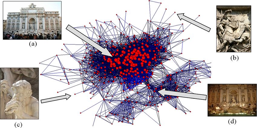
Int J Comput Vis

photographs in a 3D spatial context that gives a sense of           et al. 2003) uses proximity to transfer labels between geo-
the geometry of the underlying scene. Our approach there-           referenced photographs. An advantage of the annotation ca-
fore uses an approximate plane-based view interpolation             pabilities of our system is that our feature correspondences
method and a non-photorealistic rendering of background             enable transfer at much finer granularity; we can transfer
scene structures. As such, we side-step the more challenging        annotations of specific objects and regions between images,
problems of reconstructing full surface models (Debevec et          taking into account occlusions and the motions of these ob-
al. 1996; Teller et al. 2003), light fields (Gortler et al. 1996;   jects under changes in viewpoint. This goal is similar to that
Levoy and Hanrahan 1996), or pixel-accurate view inter-             of augmented reality (AR) approaches (e.g., Feiner et al.
polations (Chen and Williams 1993; McMillan and Bishop              1997), which also seek to annotate images. While most AR
1995; Seitz and Dyer 1996; Zitnick et al. 2004). The bene-          methods register a 3D computer-generated model to an im-
fit of doing this is that we are able to operate robustly with      age, we instead transfer 2D image annotations to other im-
input imagery that is beyond the scope of previous IBM and          ages. Generating annotation content is therefore much eas-
IBR techniques.                                                     ier. (We can, in fact, import existing annotations from pop-
                                                                    ular services like Flickr.) Annotation transfer has been also
2.5 Image Browsing, Retrieval, and Annotation                       explored for video sequences (Irani and Anandan 1998).
                                                                        Finally, Johansson and Cipolla (2002) have developed a
There are many techniques and commercial products for
                                                                    system where a user can take a photograph, upload it to a
browsing sets of photos and much research on the subject
                                                                    server where it is compared to an image database, and re-
of how people tend to organize photos, e.g., (Rodden and
                                                                    ceive location information. Our system also supports this
Wood 2003). Many of these techniques use metadata, such
                                                                    application in addition to many other capabilities (visual-
as keywords, photographer, or time, as a basis of photo or-
                                                                    ization, navigation, annotation, etc.).
ganization (Cooper et al. 2003).
    There has recently been growing interest in using geo-
location information to facilitate photo browsing. In particu-
                                                                    3 Overview
lar, the World-Wide Media Exchange (WWMX) (Toyama et
al. 2003) arranges images on an interactive 2D map. Photo-
Compas (Naaman et al. 2004) clusters images based on time           Our objective is to geometrically register large photo col-
and location. Realityflythrough (McCurdy and Griswold               lections from the Internet and other sources, and to use
2005) uses interface ideas similar to ours for exploring video      the resulting 3D camera and scene information to facili-
from camcorders instrumented with GPS and tilt sensors,             tate a number of applications in visualization, localization,
and Kadobayashi and Tanaka (2005) present an interface              image browsing, and other areas. This section provides an
for retrieving images using proximity to a virtual camera. In       overview of our approach and summarizes the rest of the
Photowalker (Tanaka et al. 2002), a user can manually au-           paper.
thor a walkthrough of a scene by specifying transitions be-            The primary technical challenge is to robustly match and
tween pairs of images in a collection. In these systems, loca-      reconstruct 3D information from hundreds or thousands of
tion is obtained from GPS or is manually specified. Because         images that exhibit large variations in viewpoint, illumina-
our approach does not require GPS or other instrumentation,         tion, weather conditions, resolution, etc., and may contain
it has the advantage of being applicable to existing image          significant clutter and outliers. This kind of variation is what
databases and photographs from the Internet. Furthermore,           makes Internet imagery (i.e., images returned by Internet
many of the navigation features of our approach exploit the         image search queries from sites such as Flickr and Google)
computation of image feature correspondences and sparse             so challenging to work with.
3D geometry, and therefore go beyond what has been possi-              In tackling this problem, we take advantage of two recent
ble in these previous location-based systems.                       breakthroughs in computer vision, namely feature-matching
    Many techniques also exist for the related task of retriev-     and structure from motion, as reviewed in Sect. 2. The back-
ing images from a database. One particular system related to        bone of our work is a robust SfM approach that reconstructs
our work is Video Google (Sivic and Zisserman 2003) (not            3D camera positions and sparse point geometry for large
to be confused with Google’s own video search), which al-           datasets and has yielded reconstructions for dozens of fa-
lows a user to select a query object in one frame of video and      mous sites ranging from Notre Dame Cathedral to the Great
efficiently find that object in other frames. Our object-based      Wall of China. Section 4 describes this approach in detail,
navigation mode uses a similar idea, but extended to the 3D         as well as methods for aligning reconstructions to satellite
domain.                                                             and map data to obtain geo-referenced camera positions and
    A number of researchers have studied techniques for au-         geometry.
tomatic and semi-automatic image annotation, and annota-               One of the most exciting applications for these recon-
tion transfer in particular. The LOCALE system (Naaman              structions is 3D scene visualization. However, the sparse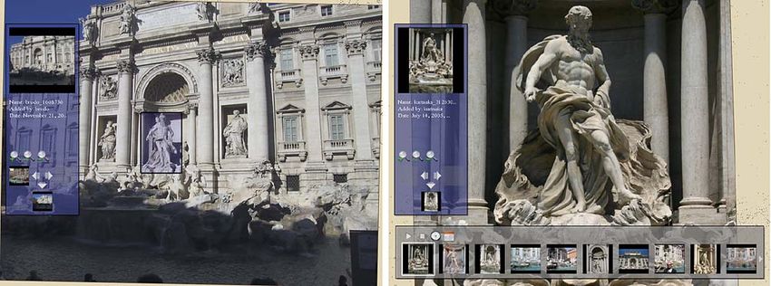
Int J Comput Vis

points produced by SfM methods are by themselves very            robust SfM procedure to recover the camera parameters. Be-
limited and do not directly produce compelling scene ren-        cause SfM only estimates the relative position of each cam-
derings. Nevertheless, we demonstrate that this sparse SfM-      era, and we are also interested in absolute coordinates (e.g.,
derived geometry and camera information, along with mor-         latitude and longitude), we use an interactive technique to
phing and non-photorealistic rendering techniques, is suffi-     register the recovered cameras to an overhead map. Each of
cient to provide compelling view interpolations as described     these steps is described in the following subsections.
in 5. Leveraging this capability, Section 6 describes a novel
photo explorer interface for browsing large collections of       4.1 Keypoint Detection and Matching
photographs in which the user can virtually explore the 3D
space by moving from one image to another.                       The first step is to find feature points in each image. We
   Often, we are interested in learning more about the con-      use the SIFT keypoint detector (Lowe 2004), because of its
tent of an image, e.g., “which statue is this?” or “when was     good invariance to image transformations. Other feature de-
this building constructed?” A great deal of annotated image      tectors could also potentially be used; several detectors are
content of this form already exists in guidebooks, maps, and     compared in the work of Mikolajczyk et al. (2005). In addi-
Internet resources such as Wikipedia8 and Flickr. However,       tion to the keypoint locations themselves, SIFT provides a
the image you may be viewing at any particular time (e.g.,       local descriptor for each keypoint. A typical image contains
from your cell phone camera) may not have such annota-           several thousand SIFT keypoints.
tions. A key feature of our system is the ability to transfer        Next, for each pair of images, we match keypoint descrip-
annotations automatically between images, so that informa-       tors between the pair, using the approximate nearest neigh-
tion about an object in one image is propagated to all other     bors (ANN) kd-tree package of Arya et al. (1998). To match
images that contain the same object (Sect. 7).                   keypoints between two images I and J , we create a kd-tree
   Section 8 presents extensive results on 11 scenes, with       from the feature descriptors in J , then, for each feature in
visualizations and an analysis of the matching and recon-        I we find the nearest neighbor in J using the kd-tree. For
struction results for these scenes. We also briefly describe     efficiency, we use ANN’s priority search algorithm, limiting
Photosynth, a related 3D image browsing tool developed by        each query to visit a maximum of 200 bins in the tree. Rather
Microsoft Live Labs that is based on techniques from this        than classifying false matches by thresholding the distance
paper, but also adds a number of interesting new elements.       to the nearest neighbor, we use the ratio test described by
Finally, we conclude with a set of research challenges for       Lowe (2004): for a feature descriptor in I , we find the two
the community in Sect. 9.                                        nearest neighbors in J , with distances d1 and d2 , then accept
                                                                 the match if dd12 < 0.6. If more than one feature in I matches
                                                                 the same feature in J , we remove all of these matches, as
4 Reconstructing Cameras and Sparse Geometry                     some of them must be spurious.
                                                                     After matching features for an image pair (I, J ), we
The visualization and browsing components of our system          robustly estimate a fundamental matrix for the pair us-
require accurate information about the relative location, ori-   ing RANSAC (Fischler and Bolles 1981). During each
entation, and intrinsic parameters such as focal lengths for     RANSAC iteration, we compute a candidate fundamental
each photograph in a collection, as well as sparse 3D scene      matrix using the eight-point algorithm (Hartley and Zis-
geometry. A few features of our system require the absolute      serman 2004), normalizing the problem to improve robust-
locations of the cameras, in a geo-referenced coordinate         ness to noise (Hartley 1997). We set the RANSAC outlier
frame. Some of this information can be provided with GPS         threshold to be 0.6% of the maximum image dimension, i.e.,
devices and electronic compasses, but the vast majority of       0.006 max(image width, image height) (about six pixels for
existing photographs lack such information. Many digital         a 1024 × 768 image). The F-matrix returned by RANSAC is
cameras embed focal length and other information in the          refined by running the Levenberg-Marquardt algorithm (No-
EXIF tags of image files. These values are useful for ini-
                                                                 cedal and Wright 1999) on the eight parameters of the F-
tialization, but are sometimes inaccurate.
                                                                 matrix, minimizing errors for all the inliers to the F-matrix.
    In our system, we do not rely on the camera or any other
                                                                 Finally, we remove matches that are outliers to the recov-
piece of equipment to provide us with location, orientation,
                                                                 ered F-matrix using the above threshold. If the number of
or geometry. Instead, we compute this information from the
                                                                 remaining matches is less than twenty, we remove all of the
images themselves using computer vision techniques. We
                                                                 matches from consideration.
first detect feature points in each image, then match feature
                                                                     After finding a set of geometrically consistent matches
points between pairs of images, and finally run an iterative,
                                                                 between each image pair, we organize the matches into
                                                                 tracks, where a track is a connected set of matching key-
8 Wikipedia,   http://www.wikipedia.org.                         points across multiple images. If a track contains more than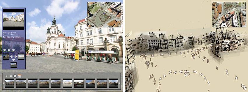
Int J Comput Vis
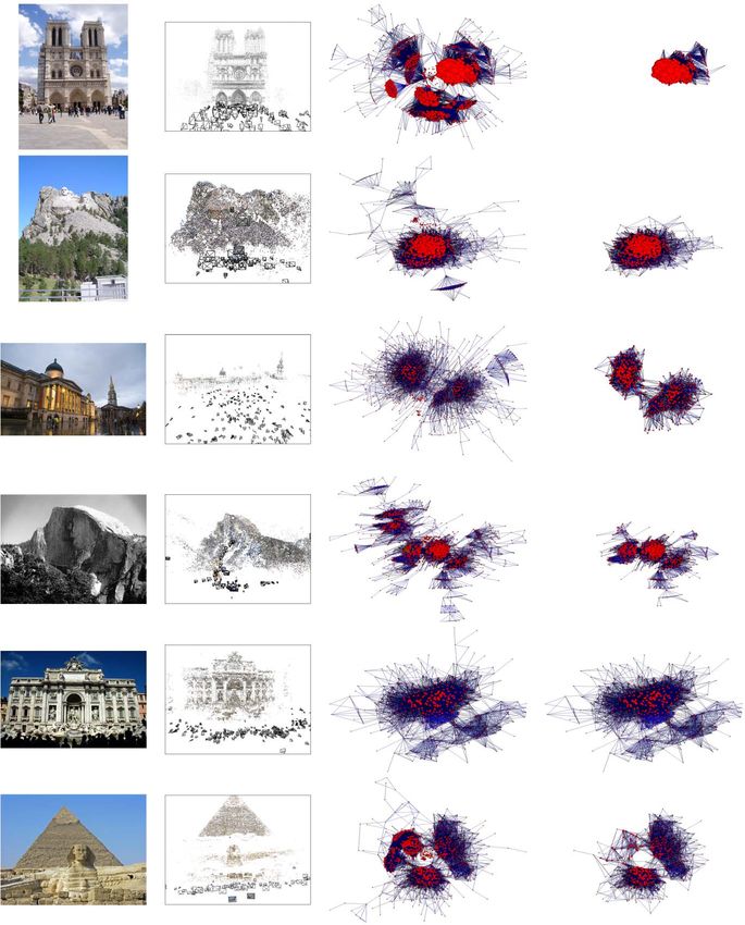
Fig. 1 Photo connectivity
graph. This graph contains a
node for each image in a set of
photos of the Trevi Fountain,
with an edge between each pair
of photos with matching
features. The size of a node is
proportional to its degree. There
are two dominant clusters
corresponding to day (a) and
night time (d) photos. Similar
views of the facade cluster
together in the center, while
nodes in the periphery, e.g., (b)
and (c), are more unusual (often
close-up) views
one keypoint in the same image, it is deemed inconsistent. to provide good initial estimates of the parameters. Rather
We keep consistent tracks containing at least two keypoints than estimating the parameters for all cameras and tracks at
for the next phase of the reconstruction procedure. once, we take an incremental approach, adding in one cam-
Once correspondences are found, we can construct an im- era at a time.
age connectivity graph, in which each image is a node and We begin by estimating the parameters of a single pair
an edge exists between any pair of images with matching of cameras. This initial pair should have a large number
features. A visualization of an example connectivity graph of matches, but also have a large baseline, so that the ini-
for the Trevi Fountain is Fig. 1. This graph embedding was tial two-frame reconstruction can be robustly estimated. We
created with the neato tool in the Graphviz toolkit.9 Neato therefore choose the pair of images that has the largest num-
represents the graph as a mass-spring system and solves for ber of matches, subject to the condition that those matches
an embedding whose energy is a local minimum. cannot be well-modeled by a single homography, to avoid
The image connectivity graph of this photo set has sev- degenerate cases such as coincident cameras. In particular,
eral distinct features. The large, dense cluster in the cen- we find a homography between each pair of matching im-
ter of the graph consists of photos that are all fairly wide- ages using RANSAC with an outlier threshold of 0.4% of
angle, frontal, well-lit shots of the fountain (e.g., image (a)). max(image width, image height), and store the percentage
Other images, including the “leaf” nodes (e.g., images (b) of feature matches that are inliers to the estimated homogra-
and (c)) and night time images (e.g., image (d)), are more phy. We select the initial image pair as that with the lowest
loosely connected to this core set. Other connectivity graphs percentage of inliers to the recovered homography, but with
are shown in Figs. 9 and 10. at least 100 matches. The camera parameters for this pair are
estimated using Nistér’s implementation of the five point al-
4.2 Structure from Motion gorithm (Nistér 2004),10 then the tracks visible in the two
images are triangulated. Finally, we do a two frame bundle
Next, we recover a set of camera parameters (e.g., rotation, adjustment starting from this initialization.
translation, and focal length) for each image and a 3D lo- Next, we add another camera to the optimization. We
cation for each track. The recovered parameters should be select the camera that observes the largest number of
consistent, in that the reprojection error, i.e., the sum of dis- tracks whose 3D locations have already been estimated,
and initialize the new camera’s extrinsic parameters using
tances between the projections of each track and its corre-
the direct linear transform (DLT) technique (Hartley and
sponding image features, is minimized. This minimization
Zisserman 2004) inside a RANSAC procedure. For this
problem can formulated as a non-linear least squares prob-
RANSAC step, we use an outlier threshold of 0.4% of
lem (see Appendix 1) and solved using bundle adjustment.
max(image width, image height). In addition to providing
Algorithms for solving this non-linear problem, such as No-
an estimate of the camera rotation and translation, the DLT
cedal and Wright (1999), are only guaranteed to find lo-
technique returns an upper-triangular matrix K which can
cal minima, and large-scale SfM problems are particularly
prone to getting stuck in bad local minima, so it is important
10 We only choose the initial pair among pairs for which a focal length
estimate is available for both cameras, and therefore a calibrated rela-
9 Graphviz—graph visualization software, http://www.graphviz.org/. tive pose algorithm can be used.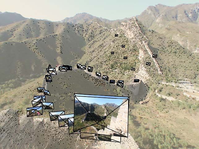
Int J Comput Vis

be used as an estimate of the camera intrinsics. We use K
and the focal length estimated from the EXIF tags of the
image to initialize the focal length of the new camera (see
Appendix 1 for more details). Starting from this initial set of
parameters, we run a bundle adjustment step, allowing only
the new camera, and the points it observes, to change; the
rest of the model is held fixed.
    Finally, we add points observed by the new camera into
the optimization. A point is added if it is observed by at least
one other recovered camera, and if triangulating the point
gives a well-conditioned estimate of its location. We esti-
mate the conditioning by considering all pairs of rays that
could be used to triangulate that point, and finding the pair
of rays with the maximum angle of separation. If this max-
imum angle is larger than a threshold (we use 2.0 degrees
                                                                   Fig. 2 Estimated camera locations for the Great Wall data set
in our experiments), then the point is triangulated. Note that
this check will tend to reject points at infinity. While points
at infinity can be very useful for estimating accurate camera      cameras to add, we first find the camera with the greatest
rotations, we have observed that they can sometimes cause          number of matches, M, to the existing 3D points, then add
problems, as using noisy camera parameters to triangulate          any camera with at least 0.75M matches to the existing 3D
points at infinity can result in points at erroneous, finite 3D    points.
locations. Once the new points have been added, we run a               We have also found that estimating radial distortion pa-
global bundle adjustment to refine the entire model. We find       rameters for each camera can have a significant effect on
the minimum error solution using the sparse bundle adjust-         the accuracy of the reconstruction, because many consumer
ment library of Lourakis and Argyros (2004).                       cameras and lenses produce images with noticeable distor-
    This procedure is repeated, one camera at a time, until no     tion. We therefore estimate two radial distortion parameters
remaining camera observes enough reconstructed 3D points           κ1 and κ2 , for each camera. To map a projected 2D point
to be reliably reconstructed (we use a cut-off of twenty           p = (px , py ) to a distorted point p  = (x  , y  ), we use the
points to stop the reconstruction process). Therefore, in gen-     formula:
eral, only a subset of the images will be reconstructed. This             2  2
                                                                           px         py
subset is not selected beforehand, but is determined by the        ρ =
                                                                     2
                                                                                  +          ,
                                                                           f           f
algorithm while it is running in the form of a termination
criterion.                                                         α = κ1 ρ 2 + κ2 ρ 4 ,
    For increased robustness and speed, we make a few mod-
                                                                   p  = αp
ifications to the basic procedure outlined above. First, af-
ter every run of the optimization, we detect outlier tracks        where f is the current estimate of the focal length (note that
that contain at least one keypoint with a high reprojec-           we assume that the center of distortion is the center of the
tion error, and remove these tracks from the optimiza-             image, and that we define the center of the image to be the
tion. The outlier threshold for a given image adapts to the        origin of the image coordinate system). When initializing
current distribution of reprojection errors for that image.        new cameras, we set κ1 = κ2 = 0, but these parameters are
In particular, for a given image I , we compute d80 , the          freed during bundle adjustment. To avoid undesirably large
80th percentile of the reprojection errors for that image,         values of these parameters, we add a term λ(κ12 + κ22 ) to the
and use clamp(2.4d80 , 4.0, 16.0) as the outlier threshold         objective function for each camera (we use a value of 10.0
(where clamp(x, a, b) = min(max(x, a), b)). The effect of          for λ in our experiments). This term discourages values of
this clamping function is that all points with a reprojection      κ1 and κ2 which have a large magnitude.
error above 16.0 pixels will be rejected as outliers, and all         Figure 2 shows an example of reconstructed points and
points with a reprojection error less than 4.0 will be kept        cameras (rendered as frusta), for the Great Wall data set, su-
as inliers, with the exact threshold lying between these two       perimposed on one of the input images, computed with this
values. After rejecting outliers, we rerun the optimization,       method. Many more results are presented in Sect. 8. For the
rejecting outliers after each run, until no more outliers are      various parameter settings and thresholds described in this
detected.                                                          section, we used the same values for each of the image sets
    Second, rather than adding a single camera at a time into      in Sect. 8, and the reconstruction algorithm ran completely
the optimization, we add multiple cameras. To select which         automatically for most of the sets. Occasionally, we found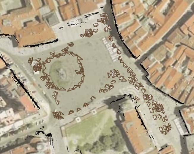
Int J Comput Vis

that the technique for selecting the initial image pair would
choose a pair with insufficient baseline to generate a good
initial reconstruction. This usually occurs when the selected
pair has a large number of mismatched features, which can
appear to be outliers to a dominant homography. When this
happens, we specify the initial pair manually. Also, in some
of our Internet data sets there are a small number of “bad”
images, such as fisheye images, montages of several differ-
ent images, and so on, which our camera model cannot han-
dle well. These images tend to be have very poor location
estimates, and in our current system these must be identified
manually if the user wishes to remove them.
    The total running time of the SfM procedure for the
data sets we experimented with ranged from about three
hours (for the Great Wall collection, 120 photos processed
and matched, and 82 ultimately reconstructed) to more than
                                                                 Fig. 3 Example registration of cameras to an overhead map. Here,
12 days (for Notre Dame, 2,635 photos processed and
                                                                 the cameras and recovered line segments from the Prague data set are
matched, and 598 photos reconstructed). Sect. 8 lists the        shown superimposed on an aerial image. (Aerial image shown here and
running time for the complete pipeline (feature detection,       in Fig. 4 courtesy of Gefos, a.s.11 and Atlas.cz)
matching, and SfM) for each data set. The running time is
dominated by two steps: the pairwise matching, and the in-
                                                                 scene, pointed downward. If the up vector was estimated
cremental bundle adjustment. The complexity of the match-
                                                                 correctly, the user needs only to rotate the model in 2D,
ing stage is quadratic in the number of input photos, but
                                                                 rather than 3D. Our experience is that it is fairly easy,
each pair of images can be matched independently, so the
                                                                 especially in urban scenes, to perform this alignment by
running time can be improved by a constant factor through
                                                                 matching the recovered points to features, such as building
parallelization. The speed of the bundle adjustment phase
                                                                 façades, visible in the image. Figure 3 shows a screenshot of
depends on several factors, including the number of pho-
                                                                 such an alignment.
tos and points, and the degree of coupling between cameras
                                                                    In some cases the recovered scene cannot be aligned to
(e.g., when many cameras observe the same set of points, the
                                                                 a geo-referenced coordinate system using a similarity trans-
bundle adjustment tends to become slower). In the future, we
                                                                 form. This can happen if the SfM procedure fails to obtain a
plan to work on speeding up the reconstruction process, as
                                                                 fully metric reconstruction of the scene, or because of low-
described in Sect. 9.
                                                                 frequency drift in the recovered point and camera locations.
                                                                 These sources of error do not have a significant effect on
4.3 Geo-Registration
                                                                 many of the navigation controls used in our explorer inter-
                                                                 face, as the error is not usually locally noticeable, but are
The SfM procedure estimates relative camera locations. The
                                                                 problematic when an accurate model is desired.
final step of the location estimation process is to optionally
                                                                    One way to “straighten out” the recovered scene is to pin
align the model with a geo-referenced image or map (such
                                                                 down a sparse set of ground control points or cameras to
as a satellite image, floor plan, or digital elevation map) so
                                                                 known 3D locations (acquired, for instance, from GPS tags
as to determine the absolute geocentric coordinates of each
                                                                 attached to a few images) by adding constraints to the SfM
camera. Most of the features of the photo explorer can work
                                                                 optimization. Alternatively, a user can manually specify cor-
with relative coordinates, but others, such as displaying an
                                                                 respondences between points or cameras and locations in
overhead map require absolute coordinates.
                                                                 an image or map, as in the work of Robertson and Cipolla
   The estimated camera locations are, in theory, related
                                                                 (2002).
to the absolute locations by a similarity transform (global
translation, rotation, and uniform scale). To determine the
                                                                 4.3.1 Aligning to Digital Elevation Maps
correct transformation the user interactively rotates, trans-
lates, and scales the model until it is in agreement with a
                                                                 For landscapes and other very large scale scenes, we can
provided image or map. To assist the user, we estimate the
                                                                 take advantage of Digital Elevation Maps (DEMs), used for
“up” or gravity vector using the method of Szeliski (2006).
                                                                 example in Google Earth12 and with coverage of most of
The 3D points, lines, and camera locations are then ren-
dered superimposed on the alignment image, using an or-
                                                                 12 Google
thographic projection with the camera positioned above the                   Earth, http://earth.google.com.
Int J Comput Vis

the United States available through the U.S. Geological Sur-         5.1 User Interface Layout
vey.13 To align point cloud reconstructions to DEMs, we
manually specify a few correspondences between the point             Figure 4 (left-hand image) shows a screenshot from the main
cloud and the DEM, and estimate a 3D similarity trans-               window of our photo exploration interface. The components
form to determine an initial alignment. We then re-run the           of this window are the main view, which fills the window,
SfM optimization with an additional objective term to fit the        and three overlay panes: an information and search pane on
specified DEM points. In the future, as more geo-referenced          the left, a thumbnail pane along the bottom, and a map pane
ground-based imagery becomes available (e.g., through sys-           in the upper-right corner.
tems like WWMX (Toyama et al. 2003) or Windows Live                      The main view shows the world as seen from a virtual
Local14 ), this manual step will no longer be necessary.             camera controlled by the user. This view is not meant to
                                                                     show a photo-realistic rendering of the scene, but rather to
4.4 Scene Representation                                             display photographs in spatial context and give a sense of
                                                                     the geometry of the true scene.
After reconstructing a scene, we optionally detect 3D line               The information pane appears when the user visits a pho-
segments in the scene using a technique similar to that of           tograph. This pane displays information about that photo,
Schmid and Zisserman (1997). Once this is done, the scene            including its name, the name of the photographer, and the
can be saved for viewing in our interactive photo explorer.          date and time when it was taken. In addition, this pane con-
In the viewer, the reconstructed scene model is represented          tains controls for searching for other photographs with cer-
with the following data structures:                                  tain geometric relations to the current photo, as described in
                                                                     Sect. 6.2.
• A set of points P = {p1 , p2 , . . . , pn }. Each point consists       The thumbnail pane shows the results of search opera-
  of a 3D location and a color obtained from one of the              tions as a filmstrip of thumbnails. When the user mouses
  image locations where that point is observed.                      over a thumbnail, the corresponding image Ij is projected
• A set of cameras, C = {C1 , C2 , . . . , Ck }. Each camera Cj      onto Plane(Cj ) to show the content of that image and how
  consists of an image Ij , a rotation matrix Rj , a translation     it is situated in space. The thumbnail panel also has con-
  tj , and a focal length fj .                                       trols for sorting the current thumbnails by date and time and
• A mapping, Points, between cameras and the points they             viewing them as a slideshow.
  observe. That is, Points(C) is the subset of P containing              Finally, the map pane displays an overhead view of scene
  the points observed by camera C.                                   that tracks the user’s position and heading.
• A set of 3D line segments L = {l1 , l2 , . . . , lm } and a map-
  ping, Lines, between cameras and the set of lines they             5.2 Rendering the Scene
  observe.
                                                                     The main view displays a rendering of the scene from the
   We also pre-process the scene to compute a set of 3D              current viewpoint. The cameras are rendered as frusta. If
planes for each camera or pair of cameras:                           the user is visiting a camera, the back face of that camera
• For each camera Ci , we compute a 3D plane, Plane(Ci ),            frustum is texture-mapped with an opaque, full-resolution
  by using RANSAC to robustly fit a plane to Points(Ci ).            version of the photograph, so that the user can see it in de-
• For each pair of neighboring cameras (i.e., cameras                tail. The back faces of the other cameras frusta are texture-
  which view at least three points in common), Ci , Cj ,             mapped with a low-resolution, semi-transparent thumbnail
  we compute a 3D plane, CommonPlane(Ci , Cj ) by us-                of the photo. The scene itself is rendered with the recovered
  ing RANSAC to fit a plane to Points(Ci ) ∪ Points(Cj ).            points and lines.
                                                                         We also provide a non-photorealistic rendering mode that
                                                                     provides more attractive visualizations. This mode uses a
5 Photo Explorer Rendering                                           washed-out coloring to give an impression of scene appear-
                                                                     ance and geometry, but is abstract enough to be forgiving
Once a set of photographs of a scene has been registered,            of the lack of detailed geometry. To generate the rendering,
the user can browse the photographs with our photo explorer          we project a blurred, semi-transparent version of each im-
interface. Two important aspects of this interface are how we        age Ij onto Plane(Cj ) and use alpha blending to combine
render the explorer display, described in this section, and the      the projections. An example rendering using projected im-
navigation controls, described in Sect. 6.                           ages overlaid with line segments is shown in Fig. 4.

                                                                     5.3 Transitions between Photographs
13 U.S.   Geological Survey, http://www.usgs.com.
14 Windows Live Local—Virtual Earth Technology Preview, http://      An important element of our user interface is the method
preview.local.live.com.                                              used to generate transitions when the user moves between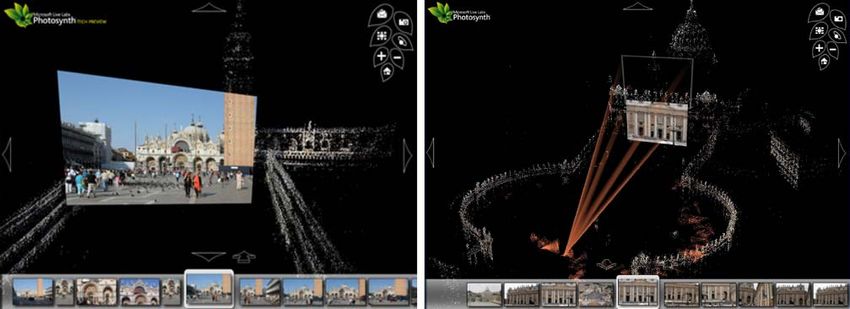
Int J Comput Vis
Fig. 4 Screenshots from the
explorer interface. Left: when
the user visits a photo, that
photo appears at full-resolution,
and information about it appears
in a pane on the left. Right:
a view looking down on the
Prague dataset, rendered in a
non-photorealistic style

photos in the explorer. Most existing photo browsing tools         Ij are imposed as edge constraints on the triangulation
cut from one photograph to the next, sometimes smoothing           (Chew 1987). The resulting constrained Delaunay triangu-
the transition by cross-fading. In our case, the geometric in-     lation may not cover the entire image, so we overlay a grid
formation we infer about the photographs allows us to use          onto the image and add to the triangulation each grid point
camera motion and view interpolation to make transitions           not contained inside the original triangulation. Each added
more visually compelling and to emphasize the spatial rela-        grid point is associated with a 3D point on Plane(Cj ). The
tionships between the photographs.                                 connectivity of the triangulation is then used to create a 3D
                                                                   mesh; we project Ij onto the mesh in order to texture map
5.3.1 Camera Motion                                                it. We compute a mesh for Ck and texture map it in the same
                                                                   way.
When the virtual camera moves from one photograph to an-               Then, to render the transition between Cj and Ck , we
other, the system linearly interpolates the camera position        move the virtual camera from Cj and Ck while cross-fading
between the initial and final camera locations, and the cam-       between the two meshes (i.e., the texture-mapped mesh for
era orientation between unit quaternions representing the          Cj is faded out while the texture-mapped mesh for Ck is
initial and final orientations. The field of view of the virtual   faded in, with the depth buffer turned off to avoid pop-
camera is also interpolated so that when the camera reaches        ping). While this technique does not use completely accu-
its destination, the destination image will fill as much of the    rate geometry, the meshes are often sufficient to give a sense
screen as possible. The camera path timing is non-uniform,         of the 3D geometry of the scene. For instance, this approach
easing in and out of the transition.                               works well for many transitions in the Great Wall data set
    If the camera moves as the result of an object selection       (shown as a still in Fig. 2, and as an animation in the video
(Sect. 6.3), the transition is slightly different. Before the      on the project website). However, missing geometry and
camera starts moving, it orients itself to point at the mean       outlying points can sometimes cause distracting artifacts.
of the selected points. The camera remains pointed at the
mean as it moves, so that the selected object stays fixed in       Planar Morphs We have also experimented with using
the view. This helps keep the object from undergoing large,        planes, rather than 3D meshes, as our projection surfaces.
distracting motions during the transition. The final orienta-      To create a morph between cameras Cj and Ck using a
tion and focal length are computed so that the selected object     planar impostor, we simply project the two images Ij and
is centered and fills the screen.                                  Ik onto CommonPlane(Cj , Ck ) and cross-fade between the
                                                                   projected images as the camera moves from Cj to Ck . The
5.3.2 View Interpolation                                           resulting in-betweens are not as faithful to the underlying
                                                                   geometry as the triangulated morphs, tending to stabilize
During camera transitions, we also display in-between im-          only a dominant plane in the scene, but the resulting arti-
ages. We have experimented with two simple techniques for          facts are usually less objectionable, perhaps because we are
morphing between the start and destination photographs: tri-       used to seeing distortions caused by viewing planes from
angulating the point cloud and using planar impostors.             different angles. Because of the robustness of this method,
                                                                   we prefer to use it rather than triangulation as the default
Triangulated Morphs To create a triangulated morph be-             for transitions. Example morphs using both techniques are
                                                                   shown in the video on our project website.15
tween two cameras Cj and Ck , we first compute a 2D
Delaunay triangulation for image Ij using the projections
of Points(Cj ) into Ij . The projections of Lines(Cj ) into        15 Photo   tourism website, http://phototour.cs.washington.edu/.
Int J Comput Vis
There are a few special cases which must be handled To make it easier to find related views such as these, we
differently during transitions. First, if the two cameras ob- provide the user with a set of “geometric” browsing tools.
serve no common points, our system currently has no ba- Icons associated with these tools appear in two rows in the
sis for interpolating the images. Instead, we fade out the information pane, which appears when the user is visiting a
start image, move the camera to the destination as usual, photograph. These tools find photos that depict parts of the
then fade in the destination image. Second, if the normal to scene with certain spatial relations to what is currently in
CommonPlane(Cj , Ck ) is nearly perpendicular to the aver- view. The mechanism for implementing these search tools
age of the viewing directions of Cj and Ck , the projected im- is to project the points observed by the current camera,
ages would undergo significant distortion during the morph. Points(Ccurr ), into other photos (or vice versa), and select
In this case, we revert to using a plane passing through the views based on the projected motion of the points. For in-
mean of the points common to both views, whose normal is stance, to answer the query “show me what’s to the left of
the average of the viewing directions. Finally, if the vanish- this photo,” we search for a photo in which Points(Ccurr )
ing line of CommonPlane(Cj , Ck ) is visible in images Ij or appear to have moved right.
Ik (as would be the case if this plane were the ground plane, The geometric browsing tools fall into two categories:
and the horizon were visible in either image), it is impossi- tools for selecting the scale at which to view the scene, and
ble to project the entirety of Ij or Ik onto the plane. In this directional tools for looking in a particular direction (e.g.,
case, we project as much as possible of Ij and Ik onto the left or right).
plane, and project the rest onto the plane at infinity. There are three scaling tools: (1) find details, or higher-
resolution close-ups, of the current photo, (2) find similar
photos, and (3) find zoom-outs, or photos that show more
6 Photo Explorer Navigation surrounding context. If the current photo is Ccurr , these tools
search for appropriate neighboring photos Cj by estimating
Our image exploration tool supports several modes for the relative “apparent size” of set of points in each image,
navigating through the scene and finding interesting pho- and comparing these apparent sizes. Specifically, to estimate
tographs. These modes include free-flight navigation, find- the apparent size of a set of points P in a image I , we project
ing related views, object-based navigation, and viewing the points into I , compute the bounding box of the projec-
slideshows. tions that are inside the image, and calculate the ratio of the
area of the bounding box (in pixels) to the area of the image.
6.1 Free-Flight Navigation We refer to this quantity as Size(P , C).
When one of these tools is activated, we classify each
The free-flight navigation controls include some of the stan- neighbor Cj as:
dard 3D motion controls found in many games and 3D view- • a detail of Ccurr if Size(Points(Cj ), Ccurr ) < 0.75 and
ers. The user can move the virtual camera forward, back, most points visible in Ccurr are visible in Cj
left, right, up, and down, and can control pan, tilt, and zoom. • similar to Ccurr if
This allows the user to freely move around the scene and
provides a simple way to find interesting viewpoints and Size(Points(Ccurr ), Cj )
0.75 < < 1.3
nearby photographs. Size(Points(Ccurr ), Ccurr )
At any time, the user can click on a frustum in the main
and the angle between the viewing directions of Ccurr and
view, and the virtual camera will smoothly move until it
Cj is less than a threshold of 10 degrees
is coincident with the selected camera. The virtual camera
• a zoom-out of Ccurr if Ccurr is a detail of Cj .
pans and zooms so that the selected image fills as much of
the main view as possible. The results of any of these searches are displayed in the
thumbnail pane (sorted by increasing apparent size, in the
6.2 Moving Between Related Views case of details and zoom-outs). These tools are useful for
viewing the scene in more detail, comparing similar views
When visiting a photograph Ccurr , the user has a snapshot of an object which differ in other respects, such as time of
of the world from a single point of view and an instant in day, season, and year, and for “stepping back” to see more
time. The user can pan and zoom to explore the photo, but of the scene.
might also want to see aspects of the scene beyond those The directional tools give the user a simple way to “step”
captured in a single picture. He or she might wonder, for left or right, i.e., to see more of the scene in a particular
instance, what lies just outside the field of view, or to the direction. For each camera, we compute a left and right
left of the objects in the photo, or what the scene looks like neighbor, and link them to arrows displayed in the infor-
at a different time of day. mation pane. To find a left and right image for camera Cj ,Int J Comput Vis
Fig. 5 Object-based
navigation. The user drags a
rectangle around Neptune in one
photo, and the system finds a
new, high-resolution photograph
we compute the average 2D motion mj k of the projections Because we only have a sparse model, however, we use a
of Points(Cj ) from image Ij to each neighboring image Ik . set of heuristics to prune the selection. If the selection was
If the angle between mj k and the desired direction (i.e., left made while visiting an image Ij , we can use the points that
or right), is small, and the apparent sizes of Points(Cj ) in are known to be visible from that viewpoint (Points(Cj )) to
both images are similar, Ck is a candidate left or right image refine the selection. In particular, we compute the 3 × 3 co-
to Cj . Out of all the candidates, we select the left of right variance matrix for the points in S ∩ Points(Cj ), and remove
image to be the image Ik whose motion magnitude mj k is all from S all points with a Mahalanobis distance greater
closest to 20% of the width of image Ij . than 1.2 from the mean. If the selection was made while not
visiting an image, we instead compute a weighted mean and
6.3 Object-Based Navigation covariance matrix for the entire set S. The weighting favors
points which are closer to the virtual camera, the idea be-
Another search query our system supports is “show me pho- ing that those are more likely to be unoccluded than points
tos of this object,” where the object in question can be di- which are far away. Thus, the weight for each point is com-
rectly selected in a photograph or in the point cloud. This puted as the inverse of its distance from the virtual camera.
type of search, applied to video in (Sivic and Zisserman
2003), is complementary to, and has certain advantages over, 6.4 Creating Stabilized Slideshows
keyword search. Being able to select an object is especially
Whenever the thumbnail pane contains more than one im-
useful when exploring a scene—when the user comes across
age, its contents can be viewed as a slideshow by pressing
an interesting object, direct selection is an intuitive way to
the “play” button in the pane. By default, the virtual camera
find a better picture of that object.
will move through space from camera to camera, pausing
In our photo exploration system, the user selects an object
at each image for a few seconds before proceeding to the
by dragging a 2D box around a region of the current photo
next. The user can also “lock” the camera, fixing it to the its
or the point cloud. All points whose projections are inside
current position, orientation, and field of view. When the im-
the box form the set of selected points, S. Our system then ages in the thumbnail pane are all taken from approximately
searches for the “best” photo of S by scoring each image in the same location, this mode stabilizes the images, making
the database based on how well it represents the selection. it easier to compare one image to the next. This mode is use-
The top scoring photo is chosen as the representative view, ful for studying changes in scene appearance as a function
and the virtual camera is moved to that image. Other images of time of day, season, year, weather patterns, etc. An exam-
with scores above a threshold are displayed in the thumb- ple stabilized slideshow from the Yosemite data set is shown
nail pane, sorted in descending order by score. An example in the companion video.16
object selection interaction is shown in Fig. 5.
Our view scoring function is based on three criteria: 6.5 Photosynth
(1) the visibility of the points in S, (2) the angle from which
the points in S are viewed, and (3) the image resolution. For Our work on visualization of unordered photo collections
each image Ij , we compute the score as a weighted sum of is being used in the Photosynth Technology Preview17 re-
three terms, Evisible , Eangle , and Edetail . Details of the com- leased by Microsoft Live Labs. Photosynth is a photo vi-
putation of these terms can be found in Appendix 2. sualization tool that uses the same underlying data (camera
The set S can sometimes contain points that the user did
not intend to select, especially occluded points that happen 16 Photo tourism website, http://phototour.cs.washington.edu/.
to project inside the selection rectangle. If we had complete 17 MicrosoftLive Labs, Photosynth technology preview, http://labs.
knowledge of visibility, we could cull such hidden points. live.com/photosynth.You can also read