Machine Learning Methods for Data Association in Multi-Object Tracking
←
→
Page content transcription
If your browser does not render page correctly, please read the page content below
Machine Learning Methods for Data Association in
                                         Multi-Object Tracking

                                         PATRICK EMAMI, University of Florida, USA
arXiv:1802.06897v2 [cs.CV] 25 Aug 2020

                                         PANOS M. PARDALOS, University of Florida, USA
                                         LILY ELEFTERIADOU, University of Florida, USA
                                         SANJAY RANKA, University of Florida, USA
                                         Data association is a key step within the multi-object tracking pipeline that is notoriously challenging due
                                         to its combinatorial nature. A popular and general way to formulate data association is as the NP-hard
                                         multidimensional assignment problem (MDAP). Over the last few years, data-driven approaches to assignment
                                         have become increasingly prevalent as these techniques have started to mature. We focus this survey solely
                                         on learning algorithms for the assignment step of multi-object tracking, and we attempt to unify various
                                         methods by highlighting their connections to linear assignment as well as to the MDAP. First, we review
                                         probabilistic and end-to-end optimization approaches to data association, followed by methods that learn
                                         association affinities from data. We then compare the performance of the methods presented in this survey,
                                         and conclude by discussing future research directions.
                                         CCS Concepts: • Computing methodologies → Tracking.
                                         Additional Key Words and Phrases: multi-object tracking; data association; machine learning; deep learning
                                         ACM Reference Format:
                                         Patrick Emami, Panos M. Pardalos, Lily Elefteriadou, and Sanjay Ranka. 2021. Machine Learning Methods for
                                         Data Association in Multi-Object Tracking. 1, 1 (May 2021), 33 pages. https://doi.org/0000001.0000001

                                         1    INTRODUCTION
                                         The assignment problem is a classic combinatorial optimization problem where the goal is to
                                         find a weighted matching within a bipartite graph such that the sum of the weights is minimized.
                                         Within the field of computer vision, it is often used as a framework for tackling data association
                                         in multi-object tracking. In this survey, we set out to reexamine the data association problem
                                         through the lens of assignment problems as a means to abstract away details and to create a clear
                                         conceptual framework for unifying the many recently proposed learning-based data association
                                         algorithms. Visual multi-object tracking is a highly complex topic, so rather than attempt to provide
                                         a comprehensive overview, we instead take a closer look at solely the association step. Later, we
                                         will suggest surveys that review other aspects of the complete multi-object tracking problem for
                                         the interested reader. In this work we argue that studying how machine learning can be used
                                         to solve data association is important for the following reasons. First, modern machine learning
                                         methods, particularly convolutional neural networks (CNNs), excel at learning discriminative
                                         Authors’ addresses: Patrick Emami, University of Florida, 432 Newell Dr, Gainesville, FL, 32611, USA, pemami@ufl.edu; Panos
                                         M. Pardalos, University of Florida, 401 Weil Hall, Gainesville, FL, 32611, USA, p.m.pardalos@gmail.com; Lily Elefteriadou,
                                         University of Florida, 512 Weil Hall, Gainesville, FL, 32611, USA, elefter@ce.ufl.edu; Sanjay Ranka, University of Florida, 432
                                         Newell Dr, Gainesville, FL, 32611, USA, sanjayranka@gmail.com.

                                         Permission to make digital or hard copies of all or part of this work for personal or classroom use is granted without fee
                                         provided that copies are not made or distributed for profit or commercial advantage and that copies bear this notice and
                                         the full citation on the first page. Copyrights for components of this work owned by others than ACM must be honored.
                                         Abstracting with credit is permitted. To copy otherwise, or republish, to post on servers or to redistribute to lists, requires
                                         prior specific permission and/or a fee. Request permissions from permissions@acm.org.
                                         © 2021 Association for Computing Machinery.
                                         XXXX-XXXX/2021/5-ART $15.00
                                         https://doi.org/0000001.0000001

                                                                                                                  , Vol. 1, No. 1, Article . Publication date: May 2021.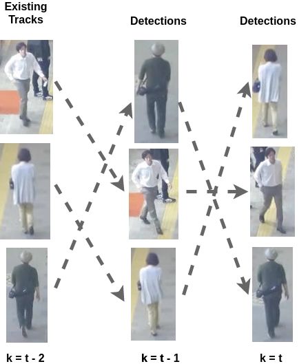
2                                                                                        P. Emami et al.

features from raw sensor inputs for computing similarities between objects, which is an integral
step for any data-driven matching task. For example, a recent study by Bergman et al. [10] showed
that a simple CNN bounding box regressor can be exploited to extend object tracks over time and
drastically reduce the number of ID switches, putting into question the efficacy of sophisticated data
association algorithms. Second, efficient probabilistic tools for approximate inference over highly
structured models, such as those that arise in data association, have long been studied and are
useful for dealing with noisy sensor measurements. Finally, there are many promising recent works
on applying machine learning to directly solve a variety of combinatorial optimization problems
[8], and it is interesting to ask whether assignment problems can be solved in a similar manner.
   Multi-object tracking with one or more sensors plays a significant role in many surveillance and
robotics applications. A tracking algorithm provides higher-level systems with the ability to make
real-time decisions based on the state of the surrounding environment and is a core part of many
scene understanding frameworks. Within intelligent transportation systems, it can be used for
increasing pedestrian safety at traffic intersections [76], moving object awareness for self-driving
cars [88], and for traffic surveillance [2, 52, 101, 138]. Multi-object tracking also has a myriad of
other applications ranging from general security systems to tracking cells in microscopy images
[70]. There are many sensor modalities that can be used for these applications; the most common
are video, radar, and LiDAR. As a motivating example, consider a vision system that tracks vehicles
and pedestrians at an urban traffic intersection. The real-time tracking data can be used for adaptive
traffic signal control to optimize the flow of traffic at that intersection. However, intersections
contain numerous challenges for multi-object tracking. Heavy traffic occupying multiple lanes and
unpredictable pedestrian motion makes for a cluttered scene with lots of occlusion, false alarms,
and missed detections. Variability in the appearance of targets caused by poor lighting and weather
conditions is especially problematic for visual tracking. On the other hand, new technologies such
as vehicle-to-infrastructure (V2I) communication enables vehicles to transmit information directly
to traffic intersections, augmenting the data collected by traffic cameras and other sensors [32].

1.1    Data Association in Multi-Object Tracking
At the core of multi-object tracking lies the measurement-to-track and track-to-track association
problems. The goal of measurement-to-track association is to identify a correspondence between a
collection of new sensor measurements and preexisting tracks (Figure 1). New measurements can
be generated by previously undetected targets, so care must be taken to not erroneously assign one
of these measurements to a preexisting track. Likewise, the measurements that stem from clutter
within the surveillance region must be identified to avoid false alarms. When there are multiple
sensors, there is also the additional problem of track-to-track association. This problem seeks to
find a correspondence between tracks that are generated by different sensors (Figure 2). Once the
optimal assignment of the multi-sensor tracks has been found, all of the tracks assigned to a single
track can be combined to produce the final estimate of that track’s state. The sensors might be
homogeneous or heterogeneous; in the latter case, the problem becomes even harder as the sensors
could produce vastly different types of data.
   Broadly speaking, algorithms for solving these two association tasks can be classified as either
single-scan, multi-scan, or batch. A single-scan algorithm only uses measurement or track informa-
tion from the most recent time step, whereas multi-scan algorithms use information from previous
and/or future time steps. Batch, or offline multi-object tracking, is an extreme version of multi-scan
where the entire sequence is available. Online multi-object tracking operates on one or a few of
the most recent scans at a time. Generally, multi-scan methods are preferable in situations where
the objects of interest are closely spaced and there are a lot of false alarms and missed detections.
However, delaying the association to leverage future information negatively affects the real-time

, Vol. 1, No. 1, Article . Publication date: May 2021.
Machine Learning Methods for Data Association in Multi-Object Tracking                                               3

          (a) Linear Assignment       (b) Linear Assignment         (c) Multidimensional Assignment

Fig. 1. Data association in multi-object tracking. a) In online tracking, new sensor detections are matched
to existing tracks at each time step by solving a linear assignment problem. The assignment hypotheses are
the colored, dashed arrows. Each arrow is annotated with the cost c i j of associating track i with detection
j. b) The optimal linear assignment. Notice how the assignment partitions the set of existing tracks and
detections. c) In batch, or offline single-sensor tracking, multiple sets of detections within a sliding window
are associated all at once with a set of existing tracks. Here, the sliding window size T is 2 and the optimal
assignment is shown. The images are taken from a random video in the MOT Challenge dataset [79].

capabilities of the tracker. The accuracy and precision of the tracks produced by multi-scan methods
are usually superior, and they offer fewer track ID switches, track breaks, and missed targets [93].
Naturally, multi-scan methods are more computationally expensive and difficult to implement than
their single-scan counterparts. The majority of the algorithms we will discuss in this survey are
online algorithms, as offline algorithms typically involve sophisticated global optimization that as
of yet is not data-driven.
   See Table 1 for a categorization of the various data association problems mapped onto assignment
problems. The easiest to solve is the bipartite matching or linear assignment problem (LAP), which
seeks to match m tracks to n detections. Usually, the problem is constrained so that each track
is assigned to exactly one measurement, but measurements are allowed to not be assigned (i.e.,
false alarms) or to be assigned to a "dummy track" (i.e., a missed detection). For multidimensional
data association, e.g., the multi-scan extension of the aforementioned linear assignment problem,
extra constraints ensure that each sensor measurement at each time step is assigned to a track
exactly once. Unfortunately, the MDAP is NP-hard for dimensions ≥ 3, whereas there exist many
polynomial-time algorithms for the LAP such as the Hungarian method [83]. We will formulate
these problems more rigorously in Section 2.

1.2   Comparison with Related Surveys
There are several related surveys to this one and in this section we will highlight their main
differences with ours. Both Poore [92] and Poore et al. [93] provide detailed treatments of how
assignment problems are useful for multi-object tracking. They only go so far as to frame assignment
problems in the context of multi-object tracking. There are a number of excellent general surveys
on multi-object tracking [72, 139]; however, their focus is on all aspects of a multi-object tracking

                                                                 , Vol. 1, No. 1, Article . Publication date: May 2021.
4                                                                                                P. Emami et al.

                                    (a)                                     (b)

Fig. 2. Track-to-track Association. There are three different sensors (circles, triangles, and diamonds)
covering the surveillance region, each maintaining two tracks. Suppose there are two ground truth objects. a)
The dashed arrows show the possible ways of associating one of the circle tracks with the tracks from the
triangle and diamond sensors. b) The best track-to-track association hypothesis. The shapes with solid lines
show all tracks, one per sensor, that have been assigned together as having originated from the same ground
truth object. Likewise for the shapes with dotted lines. The solution effectively partitions each sensor’s track
lists.

Table 1. Taxonomy of assignment problems in multi-object tracking. LAP := linear assignment problem
and MDAP := multidimensional assignment problem. The algorithms presented in this survey are mostly
for solving the various MDAPs encountered in multi-object tracking, and are generally applicable (with
modification) to both measurement-to-track and track-to-track association.

                      Measurement-to-Track Association             Track-to-Track Association
    Single-Scan       LAP (1-2 sensors), MDAP (≥ 3 sensors) LAP (2 sensors), MDAP (≥ 3 sensors)
    Multi-Scan        MDAP (≥ 1 sensors)                    MDAP (≥ 2 sensors)

solution and they do not have any emphasis on machine learning methods. A survey on appearance
matching in camera-based multi-object tracking discusses machine learning methods for improving
data association, but it does not cover the recent advances in deep learning that have become
ubiquitous in the computer vision tracking community [68]. The survey by Ciaparrone et al. [26]
provides a general overview of deep learning in multi-object tracking.

1.3    Overview of MOT Benchmarks
In this section, we will briefly review the standard multi-object tracking benchmarks. Perhaps the
most popular visual-based multi-object tracking set of benchmarks are the MOT challenges. The
MOT15 challenge was first released in 2014 and consists of 22 video sequences of pedestrians [66].
Since then, the MOT16 and MOT17 challenges have been released, with each release also improving
upon the annotation protocol and ground truth quality of the former [79]. These datasets are useful
when proposing general improvements to multi-object tracking algorithms since results from many
of the state-of-the-art trackers are publicly available for comparison. For an empirical comparison
of state-of-the-art trackers on the MOT17 benchmark, see Leal-Taixé et al. [67]. A more recent
comparison that focuses on various deep learning based trackers is available in Ciaparrone et al.
[26]. The MOT datasets are particularly challenging because scenes are filmed from both static and
moving vantage points, the density of the crowds of pedestrians is varied, and the appearances of

, Vol. 1, No. 1, Article . Publication date: May 2021.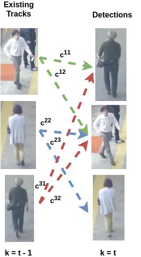
Machine Learning Methods for Data Association in Multi-Object Tracking                                               5

                           Data-Driven Combinatorial Optimization

                               Probabilistic
                                                              End-to-end Learned
                                Graphical        MCMC
                                 Models                          Assignment

                           Learning Object-Object Affinity

                                   Boosting and Metric
                                                                Deep Learning
                                        Learning

               Fig. 3. Our categorization of machine learning methods for data association.

pedestrians drastically changes between sequences. Previously, the PETS [33], TUD Stadtmitte [3],
and ETH Pedestrian [34] datasets were widely used as benchmarks. These offer a wide variety of
multi-view, indoor, and outdoor scenes, and are still useful for training and testing, despite being
less frequently used to assess state-of-the-art performance in recent works.
   Other datasets of note include the KITTI benchmark [40], which is is focused on challenges for
autonomous driving in urban environments, and contains many tasks beyond multi-object tracking
such as odometry, lane estimation, and orientation estimation. The UA-DETRAC benchmark [126]
is a large-scale traffic surveillance benchmark of 10 hours of video that was recorded at 24 different
locations in China, and contains over 8,250 vehicles that were manually annotated. For multi-sensor
traffic surveillance, the Ko-PER intersection dataset [111] offers 6 sequences collected with multiple
cameras and laser scanners; however, only 2 sequences currently have ground-truth labels.

1.4    Roadmap
Our presentation of data-driven techniques for solving data association is split into two main
sections. The first is focused on the combinatorial optimization aspect of the problem, and the
second is concerned with learning features for the assignment cost function. Prior to this, in
Section 2 we carefully present the connections between data association and assignment problems
in multi-object tracking. Section 3 will present techniques for finding optimal assignments, with a
focus on probabilistic and data-driven algorithms. Then, in Section 4 we present multiple methods
for learning features for data association. This presentation is split between algorithms used in multi-
object tracking prior to and after the introduction of deep learning. Section 5 includes a performance
comparison of methods highlighted in this survey, and Section 6 contains the conclusions. For a
visual representation of the organization of the technical contribution of the survey, see Figure 3.

2     DATA ASSOCIATION AS ASSIGNMENT
We will first formally introduce the linear assignment problem (LAP) in the context of single-sensor
data association and track-to-track association with two sensors. Following this, we will examine
certain MDAP formulations for data association problems.

2.1    Linear Assignment
Consider a scenario where there are m existing tracks and n new sensor measurements at time k,
k = 1, ...,T . We assume that there is a matrix Ck ∈ Rm×n , with entries c ki j ∈ C representing the
cost of assigning measurement j to track i at time k (Figures 1(a) and 1(b)). The goal is to find the
optimal assignment of measurements to tracks so that the total assignment cost is minimized. Using

                                                                 , Vol. 1, No. 1, Article . Publication date: May 2021.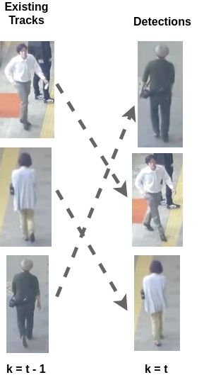
6                                                                                        P. Emami et al.

binary decision variables x i j ∈ {0, 1} to represent an assignment of a measurement to a track, we
end up with a 0-1 integer program
                                                 m Õ n
                                                       c ki j x i j
                                                Õ
                                            min                                                  (1)
                                                      x ∈X
                                                              i=1 j=1

with constraints
                                               m
                                                      x i j = 1,
                                               Õ
                                                                    j = 1, ..., n
                                               i=1
                                                n                                                   (2)
                                                         ij
                                               Õ
                                                      x = 1,        i = 1, ..., m
                                                j=1

where x ∈ X is a binary assignment matrix. There are mn constraints forcing the rows and columns
of X to sum to 1. Note that Ck is not required to be a square matrix. To capture the fact that some
sensor measurements will either be false alarms or missed detections, a dummy track is added
to the set of existing tracks, so that Ck is now an (m + 1) × n matrix. The entries in the (m + 1)th
row represent the costs of classifying measurements as false alarms. Missed detections are usually
handled by forming validation gates around the m tracks (see [13], Section 6.3). These gates can be
used to determine, with some degree of confidence, whether any of the new measurements might
have originated from a track. The canonical approach is to use elliptical gates, which are typically
computed from the covariance estimates provided by a Kalman Filter. In video-based tracking, a
similar tactic is to suppress object detections with low confidence values.
   Even though there are min(m, n)! possible assignments, many polynomial-time algorithms
exist for finding the globally optimal assignment matrix. Most famous is the O(n3 ) Hungarian
algorithm [59, 83]. Another popular method is the Auction algorithm, introduced by Bertsekas [12].
These algorithms are fast and are easy to integrate into real-time multi-object tracking solutions.
However, by only considering the previous time step when assigning measurements or tracks, we
are making a Markovian assumption about the information needed to find the optimal assignment.
In situations with lots of clutter, false alarms, missed detections, and occlusion, the performance
of these algorithms will significantly deteriorate. Indeed, it may be beneficial to instead use a
sliding window of previous and/or future track states to construct assignment costs that model
the relationship between tracks and new sensor measurements more accurately. As indicated in
Table 1, the single-scan track-to-track association problem with two sensors is also a LAP, where
m and n represent the sets of tracks maintained by each sensor. Similar methods for handling false
alarms and missed detections in data-association can be used for track-to-track association with
uneven sensor track lists. If the assignment costs are known, an optimal track assignment can be
found in polynomial-time using one of the previously mentioned algorithms.
   Instead of abandoning local data association in favor of more expensive global data association
approaches, some have proposed heuristics involving solving a cascade of LAPs [1, 130]. In particular,
DeepSORT [130] has gained in popularity due to its real-time speed and effective use of deep
association features to achieve high quality tracking.

2.2    Multidimensional Assignment
Within the single-sensor and multi-sensor tracking paradigms, there are a few different ways to
formulate measurement-to-track and track-to-track association as a MDAP (see Table 1). Each
formulation seeks to optimize slightly different criteria, but each solution technique is generally
applicable to all of them with minor modifications. We suggest further reading on the MDAP for
more details [13, 53, 92].

, Vol. 1, No. 1, Article . Publication date: May 2021.
Machine Learning Methods for Data Association in Multi-Object Tracking                                                                        7

2.2.1 Measurement-to-track association. We begin by considering the MDAP for measurement-to-
track association with one sensor given multiple scans. Let the number of scans, or the temporal
sliding window size, be given by T . Since the objective is to associate new sensor measurements
with a set of existing tracks, the resulting MDAP has T + 1-dimensions (Figure 1(c)). When T ≥ 2,
the assignment problem is NP-hard [53].
    Let the set of noisy measurements at time k be referred to as scan k and be represented by
Z k = {zki }, where i is the i th measurement of scan k, i = 1, ..., Mk . Mk is the number of measurements
in each scan, i.e., |Z k | = Mk . The main assumption we are making is that each object is responsible
for at most one measurement within each scan. We let Z T = {Z 1 , ..., ZT } represent the collection
of all measurements in the sliding window of size T .
    Let Γ be the set of all possible partitions of the set Z T . We seek an optimal partitioning γ ∗ ∈ Γ,
also called a hypothesis, of Z T into tracks. Note that a track is just an ordered set of measurements
{z 1i , z 2i , ..., zTi }; one measurement from each scan at each time step is attributed to each track. Hence,
a partition γ represents a valid collection of tracks that adhere to the MDAP constraints. Now, we
define γ j to be the j th track in γ . Following this, we can define a cost for each track γ j in a partition
as c i 1,i 2, ...,iT , where the indices i 1 , i 2 , ..., iT indicate which measurements from each scan belong
to this particular track. This represents the cost of track j being assigned measurement i from
scan 1, measurement i from scan 2, and so on. Crucially, the multidimensional constraints prevent
measurements from being assigned to two different tracks and ensure that each measurement is
matched to a track. If we use binary variables ρ i 1,i 2, ...,iT ∈ {0, 1} to indicate if a track is present in
a partition, then we can represent the MDAP objective as
                                                  M1
                                                  Õ              MT
                                                                 Õ
                                           min             ...           c i 1,i 2, ...,iT ρ i 1,i 2, ...,iT                                (3)
                                           γ ∈Γ
                                                  i 1 =1         iT =1

with constraints
                              M1
                              Õ              MT
                                             Õ
                                       ...            ρ i 1,i 2, ...,iT = 1;                   i 1 = 1, ..., M 1
                              i 2 =1         iT =1
                              M1
                              Õ              MT
                                             Õ
                                       ...            ρ i 1,i 2, ...,iT = 1;                   i 2 = 1, ..., M 2
                              i 1 =1         iT =1                                                                                          (4)
                                                                         ..                         ..
                                                                          .                          .
                            M1
                            Õ              MÕ
                                            T −1

                                     ...              ρ i 1,i 2, ...,iT = 1;                   iT = 1, ..., MT .
                            i 1 =1         iT −1 =1
The solution ρ to this MDAP is the multidimensional extension of the binary assignment matrix.
Simply, one may consider ρ as being a multidimensional array with binary entries, such that the
sum along each dimension is 1. Similarly to the LAP, we can augment each scan by including a zk0
dummy measurement in the set of detections at time k to address false alarms. This is useful for
identifying track birth and track death as well, but care should be taken when defining the cost
for assigning measurements as false alarms or missed detections to avoid high numbers of false
positives and false negatives.
   It is common to solve for an approximate solution within a fixed-sized sliding window T , then
shift the sliding window forward in time by t < T so that the new sliding window overlaps with
the old region. This allows for tracks to be linked over time, and it provides a compromise between
“offline" tracking, when T is set to the length of an entire sequence of measurements, and "online"
tracking, when T = 1.

                                                                                          , Vol. 1, No. 1, Article . Publication date: May 2021.
8                                                                                                                          P. Emami et al.

2.2.2 Track-to-track association. The other form of the MDAP we are interested in is multi-sensor
association with S ≥ 3 sensors. This scenario is common in centralized tracking systems, where
sensors that are distributed around a surveillance region report raw measurements to a central
node [14, 110]. When each sensor sends its local tracks to a central node for track association and
fusion, a MDAP must be solved. In this case, the dimensionality of the MDAP is equal to S, and
hence, is NP-hard. Multi-scan track-to-track association with two sensors is also a MDAP, as well
as multi-scan multi-sensor measurement-to-track association (Table 1).
     Following [30], in this scenario there are S ≥ 3 sensors, each maintaining a set of local tracks
and using a sliding window of size T ≥ 1. We define X ks = {x ki,s }, s = 1, ..., S, to represent
the set of track state estimates produced by sensor s at time k. We have i = 1, ..., Ns , where
Ns is the number of tracks being maintained by sensor s and x ki,s interpreted as the i th track of
sensor s at scan k. Then, for each sensor, we have X T ,s = {X 1s , ..., XTs }, which represents the
collection of track state estimates within the sliding window. We seek an optimal partitioning
γ ∗ ∈ Γ of X T = {X T ,1 , ..., X T ,S } of tracks over all scans and sensors that minimizes the total
assignment cost, and we can define a partial assignment hypothesis in a partition γ as γ l =
{{x 1j,1 , x 1j,2 , ..., x 1j, Ns }, ..., {xTj,1 , xTj,2 , ..., xTj, Ns }}. In words, this states that the j th track of sensor 1
from scan 1, j th track of sensor 2 from scan 1, and so on, all correspond to the same underlying
track l in scan 1. Likewise, this interpretation extends for all subsequent scans. As a quick example,
suppose that there are 3 sensors each maintaining 3 tracks, and that T = 1. Then a potential
hypothesis γ , or assignment, is {{x 1,1 , x 2,2 , x 1,3 }, {x 2,1 , x 1,2 , x 2,3 }, {x 1,3 , x 2,3 , x 3,3 }}. This hypothesis
makes the claim that track 1 from sensor 1, track 2 from sensor 2, and track 1 from sensor 3 all were
generated by "true" track 1. The assignments for the other two tracks can be identified similarly.
Note that the number of "true" targets in the surveillance region must either be known a priori or
estimated. Considering the simplest case of T = 1, we can write the cost for a partial hypothesis as
c i 1,i 2, ...,i Ns . Increasing T to include more than one scan corresponds to adding extra dimensions
to the problem. We can use binary variables as before, ρ i 1,i 2, ...,i Ns ∈ {0, 1}, to indicate whether a
particular partial hypothesis is present in γ . The MDAP can then be written as
                                                    N1
                                                    Õ               Ns
                                                                    Õ
                                             min             ...             c i 1,i 2, ...,i Ns ρ i 1,i 2, ...,i Ns                  (5)
                                             γ ∈Γ
                                                    i 1 =1         i Ns =1

with constraints
                                N1
                                Õ               Ns
                                                Õ
                                         ...              ρ i 1,i 2, ...,i Ns = 1;                   i 1 = 1, ..., N 1
                                i 2 =1         i Ns =1
                                N1
                                Õ               Ns
                                                Õ
                                         ...              ρ i 1,i 2, ...,i Ns = 1;                   i 2 = 1, ..., N 2
                                i 1 =1         i Ns =1                                                                                (6)
                                                                               ..                          ..
                                                                                .                           .
                               N1
                               Õ               N
                                               Õ s −1

                                       ...                ρ i 1,i 2, ...,i Ns = 1;                   i Ns = 1, ..., Ns .
                              i 1 =1         i Ns −1 =1

As with the multi-scan data association problem, the solution takes the form of a multidimensional
binary array. As before, the number of potential assignment hypotheses in a MDAP can be reduced
with gating. Even with gating, solving a MDAP for real-time tracking is infeasible. An analysis on the
number of local minima in MDAPs with random costs shows that it increases exponentially in the
number of dimensions [43]. Notably, the MDAP is closely related to other NP-Hard combinatorial

, Vol. 1, No. 1, Article . Publication date: May 2021.
Machine Learning Methods for Data Association in Multi-Object Tracking                                               9

optimization problems, such as Maximum-Weight Independent Set and Set Packing [27]. In the next
subsection, we will show how the costs can be interpreted as probabilities; this will help motivate
the use of approximate inference techniques for finding maximum a posteriori (MAP) solutions
to MDAPs. However, we will begin our discussion of optimization approaches in Section 3 with
techniques that do not require any assumptions about the nature of the cost function.

3     ALGORITHMS FOR FINDING OPTIMAL ASSIGNMENTS
We begin by briefly reviewing non-probabilistic optimization algorithms for solving the data
association problem. These mostly fall into the category of offline data association. Next, our focus
will shift to methods with a machine learning flavor. The techniques discussed in this section are
quite general, and in most cases can be used for both the measurement-to-track and track-to-track
MDAPs with proper modification. The majority of these algorithms are developed for online MOT.
We conclude by reviewing recent progress on end-to-end data association, which attempt to replace
the combinatorial aspects of the problem with data-driven methods.

3.1    Non-probabilistic Algorithms
3.1.1 Search Algorithms. Heuristically searching through the space of valid solutions within a
time limit is an attractive way of ensuring both real-time performance and that a good local optima
will be discovered. A search procedure for a MDAP takes as input a problem instance in the form of
Equation 3 or Equation 5 and constructs a valid solution γ by adding each legal partial assignment
incrementally. The most well-known method, the Greedy Randomized Adaptive Search Procedure
(GRASP), was originally introduced for multi-sensor multi-object tracking [84].
   Other greedy search algorithms have been proposed [90, 105] based on the semi-greedy track
selection (SGTS) algorithm [19]. SGTS-based algorithms first perform the usual greedy assignment
algorithm step of sorting potential tracks by track score, then they generate a list of candidate
hypotheses and return the locally optimal result. The main strength of search algorithms appear to
be their simplicity and the extent to which they are embarrassingly parallel.
   For a survey of research on GRASP for optimization, see Resende [98].
3.1.2 Lagrangian Relaxation. The multidimensional binary constraints 4 and 6 pose a significant
challenge; a standard technique is to relax the constraints so that a polynomial-time algorithm can
be used to find an acceptable sub-optimal solution. The existence of O(n3 ) algorithms [12, 59, 83]
for the LAP suggests that if the constraints can be relaxed, a reasonably good solution to the MDAP
should be obtainable within an acceptable amount of time. Indeed, Lagrangian relaxation algorithms
for association in multi-object tracking [29, 30] involve iteratively producing increasingly better
solutions to the MDAP by successively solving relaxed LAPs and reinforcing the constraints.
   A parallel implementation of this method for the K-best case was developed [94, 95], which
enables efficient implementations of MHT algorithms. A variation on this approach using dual
decomposition has been proposed as well [63].
   Lagrangian relaxation has also been used to convert Equation 3 into a global network flow
problem [18]. The motivation behind this approach is a desire to incorporate higher-order motion
smoothness constraints, beyond what is capable when only considering pairwise costs in multi-scan
problems. The minimum-cost network flow problem that results from the relaxation can be solved
in polynomial-time; updates to the Lagrange multipliers enforcing the constraints are handled by
subgradient methods. In the next subsection, we go into more detail on network optimization, one
of the leading approaches to solving multi-object tracking association problems.

3.2    Probabilistic Graphical Models

                                                                 , Vol. 1, No. 1, Article . Publication date: May 2021.
10 P. Emami et al.
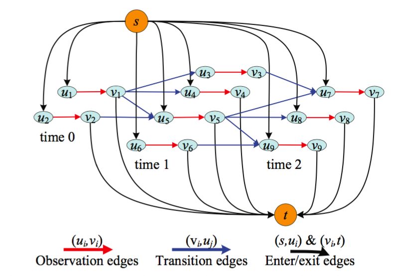
Fig. 4. A network flow graph for multi-scan data association (three scans depicted). The black arcs represent
enter/exit edges for a potential track. The red arcs are measurement/observation edges, and the blue arcs are
transition edges between measurements. Reproduced from [140] with permission.
3.2.1 Network Optimization. A popular approach (Equation 3) in the multi-object tracking com-
puter vision community is to transform the data association problem into finding a minimum-cost
network flow [9, 18, 22, 50, 91, 103, 119, 122, 131, 137, 140]. In the corresponding network, detections
at each discrete time step generally become the nodes of the graph, and a complete flow path
represents a target track, or trajectory. The amount of flow sent from the source node to the sink
node corresponds to the number of targets being tracked, and the total cost of the flow on the
network corresponds to the log-likelihood of the association hypothesis. The globally optimal
solution to a minimum-cost network flow problem can be found in polynomial-time, e.g., with the
push-relabel algorithm.
Another benefit of using minimum-cost network flow is that the graph can be constructed to
significantly reduce the potential number of association hypothesis by limiting transition edges
between nodes with a spatiotemporal nearness criteria, similar to gating. Furthermore, occlusion
can be explicitly modeled by adding nodes to the graph corresponding to the case where a target is
partially or fully occluded by another target for some amount of time. A sliding window approach
can be used for real-time performance, rather than using the complete history of previous detections.
To help illuminate the mapping from Equation 3 to a network flow problem, we adapt the following
equations from Zhang et al. [140], rewritten using the notation from Section 2.
Recall that we defined a data association hypothesis γ as a partitioning of the set of all available
measurements Z T . Then, a MAP formulation of the MDAP for data association is given by
γ ∗ = arg max P(Z T | γ )
Ö
P(Tm )
γ ∈Γ Tm ∈γ (7)
s.t. Tm ∩ Tn = ∅, ∀m , n
where the product over tracks in the objective reflects an assumption of track motion independence,
and the potentially prohibitive constraint guarantees that no two tracks ever intersect. It is possible
to derive the measurement likelihood using Equation 22; in Zhang et al. [140], it is factored as
, Vol. 1, No. 1, Article . Publication date: May 2021.Machine Learning Methods for Data Association in Multi-Object Tracking 11
P(Z T | γ ) = z P({z ∈ Z T } | γ ), where each term in this product is a Bernoulli distribution with
Î
parameter β encoding the probability of false alarm and missed detection. The track probabilities
P(Tm ) are modeled as Markov chains to capture track initialization, termination, and state transition
probabilities. A network flow graph can now be defined as a graph with source s and sink t as
follows. For every measurement zki ∈ Z T , create two nodes ur , vr , create an arc (ur , vr ) with cost
c(ur , vr ) and flow f (ur , vr ), an arc (s, ur ) with cost c(s, ur ) and flow f (s, ur ), and an arc (vr , t) with
cost c(vr , t) and flow f (vr , t). For every transition P(zki +1 | zki ) , 0, create an arc (vr , us ) with
cost c(vr , us ) and flow f (vr , us ). An example of such a graph is given in Figure 4. The flows f are
indicator functions defined by
(
1 if ∃Tm ∈ T , Tm starts from ur
f (s, ur ) =
0 otherwise
(
1 if ∃Tm ∈ T , Tm ends at vr
f (vr , t) =
0 otherwise
( (8)
1 if ∃Tm ∈ T , zki ∈ Tm
f (ur , vr ) =
0 otherwise
(
1 if ∃Tm ∈ T , zki +1 comes after zki in Tm
f (vr , us ) =
0 otherwise
and the costs are defined as
c(s, ur ) = − log P start (zki ) c(vr , t) = − log Pend (zki )
βr (9)
c(ur , vr ) = log c(vr , us ) = − log Plink (zki +1 | zki ),
1 − βr
and can be derived by taking the logarithm of Equation 7; see Section 3.2 of [140] for more details.
The minimum cost flow through the network corresponds to the assignment γ ∗ with the maximum
log-likelihood.
Quite a few variations on this model have been proposed in the literature. In one case, a subgraph
is created for each track in the surveillance region and occlusion is modeled by adding special
nodes to the graphs [50]. A linear programming relaxation with a sliding-window heuristic then
enables approximate global solutions to be found in real-time. A limitation of this approach is the
requirement of knowing a priori the number of tracks in the surveillance region, as well as the
poor worst-case complexity of the simplex method. Another work further optimizes the approach
introduced in Zhang et al. [140] to reduce the run-time complexity [91]. In a more drastic departure
from previous works in this direction, the problem has also been formulated as a K-shortest paths
through a flow graph [9]. One argument against the previously discussed network flow models is
that they exhibit an over-reliance on appearance modeling and pairwise costs [27]. They offer a
variation on the network flow approach that uses a more general cost function. In Section 4, we
will go over the details of works that propose a variety of machine learning techniques to obtain
the link costs (Equation 9) in network flow graphs. Network optimization techniques offer a good
trade-off between complexity, ease of implementation, and performance.
3.2.2 Conditional Random Fields. Probabilistic graphical models provide us with a powerful set of
tools for modeling spatiotemporal relationships amongst sensor measurements in data association
and amongst tracks in track-to-track association. Indeed, conditional random fields (CRFs), a class
of Markov random fields [62], have been used extensively for solving MDAPs in visual tracking
[22, 64, 82, 88, 135, 136]. A CRF is an undirected graphical model, often used for structured prediction
, Vol. 1, No. 1, Article . Publication date: May 2021.12 P. Emami et al.
tasks, that can represent a conditional probability distribution between sets of random variables.
CRFs are well-known for their ability to exploit grid-like structure in the underlying probabilistic
model.
We define a CRF over a graph G = (V , E) with nodes xv ∈V ∈ X such that each node emits a label
y ∈ Y . For simplicity of notation, we refer to nodes as x and omit the subscript. The labels take
on values from a discrete set, e.g., {0, 1}; in the context of multi-object tracking, a realization of
labels y usually corresponds to an assignment hypothesis. A key theorem concerning random fields
states that the probability distribution being modeled can be written in terms of the cliques c of the
graph [44]. For example, in chain-structured graphs, each pair of nodes and corresponding edge is
a clique.
CRFs, like the probabilistic network flow models discussed in the previous subsection, are
essentially a tool for modeling probabilistic relationships between a collection of random variables.
They require a separate optimization process for handling training and inference (such as the
graph cut algorithm [15] or message passing algorithms). We will focus on presenting how the
data association problem is mapped onto a CRF and direct the reader to other sources [15] for
details on how exactly approximate inference is carried out for these models. One of the benefits of
using graphical models is that we have the flexibility to construct our graph using either sensor
measurements, tracklets (measurements that are partially associated to form a "sub"-track), or full
tracks. Tracklets are a common choice for CRFs since they give an attractive hierarchical quality
to the tracking solution; low-level measurements are first associated into tracklets via, e.g., the
Hungarian algorithm, and then stitched together into full tracks via a CRF. By working at a higher
level of abstraction, the original MDAP constraints 4 and 6 are modified slightly; all that is needed
at the higher level is to ensure that each tracklet is only associated to one and only one track. This
can also help reduce processing time for running in real-time.
Each clique c in the graph has a clique potential ψc associated with it; usually, the clique potentials
are written as the product of unary terms ψs and pairwise terms ψs,t . It is common to assume
⊺
a log-linear representation for the potentials, i.e., ψc = exp(w c ϕ(x, yc )). Note that the implied
normalization term in Equation 10 can be omitted when solving for the maximum-likelihood
labeling y for a particular set of observations x, such that
Ö
P(y | x, w) ∝ ψc (yc | x, w)
c
Ö Ö (10)
∝ ψs (ys | x, w) ψs,t (ys , yt | x, w).
s ∈V s,t ∈E
Features ϕ must be provided (or can be extracted from data with supervised or unsupervised learn-
ing) and weights w are learned from data. The observations x can be either sensor measurements
(for data association) or sensor-level tracks (for track-to-track association). The Markov property
of CRFs can be interpreted in the context of multi-object tracking as assuming that the assignment
of the observations to tracks within a particular spatiotemporal section of the surveillance region
is independent of how they are assigned to tracks elsewhere—conditional on all observations. This
adds an aspect of local optimality and, in a way, embeds similar assumptions as a gating heuristic.
A solution to Equation 10, i.e., the maximum-likelihood set of labels y, can be used as a solution to
the corresponding MDAP.
As is common with CRFs, the problem of solving for the most likely assignment hypothesis
is cast as energy minimization. The objective to minimize is an energy function, computed by
summing over the clique potentials; each potential is interpreted as contributing to the energy
of the assignment hypothesis. Each clique consists of a set of vertices and edges, where each
vertex is a pair of tracklets that could potentially be linked together. The corresponding labels
, Vol. 1, No. 1, Article . Publication date: May 2021.Machine Learning Methods for Data Association in Multi-Object Tracking 13
for each vertex take values from the set {0, 1} and indicates whether a pair of tracklets are to be
linked or not. The energy term for each clique is decomposed into the sum of a unary term for the
vertices and a pairwise term for the edges. In one instance, the weights w are learned with the
RankBoost algorithm [135]. Other techniques for learning the parameters of a CRF that maximize
the log-likelihood of the training data include iterative scaling algorithms [62] and gradient based
techniques. In Section 4, we will examine the problem of learning weights for assignment costs in
more detail. The features used to construct these terms include appearance, motion, and occlusion
information, among others. CRF and network optimization-based trackers are by nature global
optimizers, and must be run with a temporal sliding-window to get near real-time performance.
For example, extensions to the generic CRF formulation have been developed that enable it to run
in real-time [136].
A particular CRF formulation, Near Online Multi-Target Tracking (NOMT) [22], also builds its
graph of track hypotheses using tracklets. The novelty of this work is in the use of an affinity
measure between detections called the Aggregated Local Flow Descriptor, and in the specific form
of the unary and pairwise terms in the energy function of the CRF. Inference in the CRF is sped
up by first analyzing the structure of the graphical model so that independent subgraphs can be
solved in parallel.
Other variations on the approaches above have been seen as well. In one such work, the energy
term of a CRF is augmented with a continuous component to jointly solve the discrete data associa-
tion and continuous trajectory estimation problems [82]. Another study embedded a factor graph
in the CRF to add more structure and help model pairwise associations explicitly [46]. Based on
the insight that the size of the bounding box is an indicator of object localization accuracy, asym-
metric pairwise terms are added to the CRF that take this idea into account for better uncertainty
management [141].
In the sequel, we will investigate how factor graphs, the belief propagation inference algorithm,
and its variants can be used to solve the MDAP. To summarize, applying CRFs to a specific multi-
object tracking problem involves defining how the graphical model will be constructed from the
sensor data, specifying an objective function, selecting or learning features for the terms within
the objective function, training the model to learn the weights, and then performing approximate
inference to extract the predicted assignment hypothesis.
3.2.3 Belief Propagation. In this section, we highlight recent work that formulate the association
problems as MAP inference and use belief propagation (BP) or one of its variants to obtain a solution.
Chen et al. [20, 21] showed the effectiveness of BP at finding the MAP assignment hypothesis for the
single and multi-sensor data association problems. BP is a general message-passing algorithm that
can carry out exact inference on tree-structured graphs and approximate inference on graphs with
cycles, or "loopy" graphs. The types of graphs under consideration are once again Markov random
fields, albeit more general ones than the ones discussed in the previous subsections. Indeed, BP can
be used on graphs that model joint distributions P(x) = P(x 1 , x 2 , ..., x N ) that can be factorized into
a product of clique potentials. As before, the clique potentials are assumed to be factorizable into
pairwise terms. Therefore, for cliques c, we have
Ö
P(x) ∝ ψc (x c )
c
Ö Ö (11)
∝ ψs (x s ) ψs,t (x s , x t ).
s ∈V s,t ∈E
It is common to use factor graphs to explicitly encode dependencies between variables. A factor
graph decomposes a joint distribution into a product of several local functions f j (X j ), where each
, Vol. 1, No. 1, Article . Publication date: May 2021.14 P. Emami et al.
X j is some subset of {x 1 , x 2 , ..., x N }. The graph is bipartite and has nodes x (i.e., discrete random
variables) and factors (i.e., dependencies) f ∈ F , and edges between the nodes and factors. For
example, the graph of д(x 1 , x 2 , x 3 ) = f A (x 1 )f B (x 2 , x 3 )fC (x 1 , x 3 ) has factors f A , f B , and fC and nodes
x 1 , x 2 , x 3 . The joint distribution for a factor graph can be written similarly to Equation 11 as
Ö Ö
P(x) ∝ ψs (x s ) ψ f (x η f ), (12)
s ∈V f ∈F
where η f represents the set of nodes x that are connected to factor f .
Parallel message-passing algorithms, such as BP, operate by having each node of the graph
iteratively send messages to its neighbors simultaneously. We define messages from a node x s to
its neighbors x t ∈ N (s) as µ s→t (x s ). In a factor graph, the set of neighbors N (s) for a node x s are
its corresponding factors. The max-product algorithm is useful for finding the MAP configuration
x ∗ = {x ∗ s | s ∈ V } which corresponds to the best assignment hypothesis γ ∗ . In this algorithm,
messages are computed recursively in general pairwise Markov random fields by
Ö
µ s→t (x s ) = max ψ (x t )ψs,t (x s , x t ) µ ξ →t (x t ) (13)
xt
ξ ∈N (t )\s
and at convergence, each x s∗ can be calculated by
Ö
x s∗ = arg max ψs (x s ) µ ξ →s (x s ) (14)
x s ∈X ξ ∈ nbr(s)
for neighborhood set nbr(s). These updates are not guaranteed to converge for graphs with cycles,
and even if they do, they may not compute the exact MAP configuration [20]. See Williams et al.
[127] for a proof of convergence of loopy belief propagation (LBP) for data association. LBP simply
applies the BP updates repeatedly until the messages all converge; interestingly, LBP has been
shown to perform favorably in practice for association tasks [78, 128, 129]. An improvement over
the max-product algorithm for LBP is tree-reweighted max-product [117]. This algorithm is used
for data association to output a provably optimal MAP configuration or acknowledge failure [20].
The key idea of the tree-reweighted max-product algorithm is to represent the original problem as
a combination of tree-structured problems that share a common optimum [20].
To illustrate the use of BP for solving MDAPs, we will present the graphical model formulation
from Zhu et al. [142] for multi-sensor multi-object track-to-track association. The structure of
the graphical model is decided on-the-fly by producing sets of independent association clusters
consisting of multi-sensor tracks that could plausibly be associated with each other. This is accom-
plished by computing elliptical gates around each track and clustering together all such tracks
whose gates overlap, using e.g., kinematic information. The nodes of the graph are the track state
estimates for T = 1 and S ≥ 3 sensors (Section 2), x i, j | x i, j ∈ X 1 = {X 1,1 , X 1,2 , ..., X 1,S } , where
each x i, j is the i th track state estimate from sensor j, i = 1, ..., N j and j = 1, ..., S. Edges only exist
between nodes from different sensors when their elliptic gates overlap. A random variable Y i, j
corresponding to each node x i, j is defined as a vector of S − 1 dimensions and stores the indexes of
the tracks from the other sensors associated with the i th track from sensor j. The node potentials
are defined as ψ x i, j (Y i, j ) = exp(ρ) where ρ is the sum of pair-wise costs, given by Equation 23.
Using the notation Yki, j to denote the k th entry of the S − 1-dimensional vector Y i, j , (the index of
the local track from sensor k), the edge potentials can be defined to ensure that each track from
, Vol. 1, No. 1, Article . Publication date: May 2021.Machine Learning Methods for Data Association in Multi-Object Tracking 15
each sensor is associated once and only once by
0 p = n, q , l
ψ x l,m →x n,o (Ynl,m = p, Yln,o = q) = 0 p , n, q = l
(15)
1 otherwise.
If w u,v is the Mahalanobis distance between two tracks u, v, then messages between nodes can be
initialized as (
n,o exp(w u=(l,m);v=(n,o) ) if q = l
µ x l,m →x n,o (Yl = q) = (16)
1 otherwise.
Then, repeated applications of Equations 13 and 14 until the Y i, j s converge will produce the MAP
solution.
This approach has been extended for an unknown number of targets and multiple sensors [77]
and applied to a multistatic sonar network [78]. For a general overview of graph techniques for the
data association problem, including BP, see Chong [23].
3.3 Markov Chain Monte Carlo
A principled approach to sampling from a complex, potentially high-dimensional distribution is
Markov Chain Monte Carlo (MCMC). MCMC methods construct a Markov chain on the state
space X whose stationary distribution π ∗ is the target distribution. Decorrelated samples drawn
from the chain can be used for approximate inference, i.e., integrating with respect to π ∗ . This
is useful in the context of assignment problems for multi-object tracking when the goal is to
estimate a posterior distribution over assignment hypotheses, from which a MAP hypothesis can
be extracted. The Metropolis-Hastings algorithm has been used extensively for data association in
single and multi-sensor scenarios [7, 35, 85, 89]. Recently, a Gibbs sampler was derived for efficient
implementations of the Labeled Multi-Bernoulli filter, which jointly addresses the data association
and state estimation problems for single and multi-sensor scenarios [99, 116]. We omit detailed
descriptions of the Metropolis-Hastings and Gibbs sampling algorithms, and instead refer the reader
to relevant work [85, 116].
MCMC is applied to the MDAP for data association (referred to as MCMCDA) and track-to-
track association by designating the state space of the Markov chain to be all feasible assignment
hypotheses and the stationary distribution of the Markov chain to be the posterior P(γ | Z T ) or
P(γ | X T ). A MAP assignment hypothesis γ ∗ for the data association problem is:
T
f
P(γ | Z T ) ∝ P(Z T | γ ) pzzt (1 − pz )c t pddt (1 − pd )дt λbat λ ft
Ö
(17)
t =1
γ ∗ = arg max P(γ | Z T ). (18)
γ
Here, we define the survival probability as pz and the detection probability as pd . The number of
targets at time t − 1 is et −1 , the number of targets that terminate at time t is zt , and c t = et −1 − zt is
the number of targets from time t − 1 that have not terminated at time t. We set at as the number of
new targets at time t, dt as the number of actual target detections at time t, and дt = c t + at − dt as
the number of undetected targets. Finally, let ft = nt − dt be the number of false alarms, λb be the
birth rate of new objects, and λ f be the false alarm rate. Note that for the general case of unknown
numbers of targets, the multi-scan MCMCDA will find an approximate solution of unknown quality
at best. A bound on the quality of the approximation for the single-scan fixed target MCMCDA has
been derived [85].
, Vol. 1, No. 1, Article . Publication date: May 2021.16 P. Emami et al.
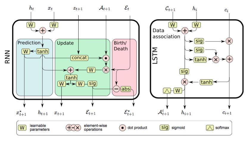
Fig. 5. An LSTM cell designed for multi-scan single-sensor data association (right). The input at each time
step is the matrix of pairwise distances Ct +1 , along with the previous hidden state ht and cell state c t .
The output Ait +1 of the data association cell is a vector of assignment probabilities for each target and
all available measurements, obtained by a log-softmax operation, and is subsequently fed into the state
estimation recurrent network (left). The LSTM’s nonlinearities and memory are believed to provide the means
for learning efficient solutions to the data association problem. Best viewed in color. Reproduced from [81]
with permission.
A Metropolis-Hastings algorithm for Equation 17 is as follows [85]. The proposal distribution
q is associated with five types of moves, for a total of eight moves; a birth/death move pair, a
split/merge move pair, an extension/reduction move pair, a track update move, and a track switch
move. A move is accepted with acceptance probability A(γ , γ ′), where
π (γ ′)q(γ ′, γ )
A(γ , γ ) = min 1,
′
. (19)
π (γ )q(γ , γ ′)
Assuming a uniform proposal distribution q, the proposal distribution terms in the numerator and
denominator cancel. The stationary distribution π (γ ) is P(γ | Z T ) from Equation 17. Implementation
details and descriptions of each type of move can be found in Section V-A of Oh et al. [85]. Extensions
to this algorithm have been proposed [7] to add a sliding-window version and to reduce the number
of types of moves to three. For visual tracking [7], appearance information is fused with kinematic
information to help improve performance. Sparse representations of detections and kinematic
information have been used to define an energy objective that MCMCDA approximately optimizes
[35]. This work deviates from its predecessors by allowing moves to be done not only forward in
time, but also backwards to explore the solution space more efficiently. The use of a sliding-window
is once again crucial, enabling the trade-off between solution quality and a faster run-time.
3.4 End-to-end Data Association
Neural networks have a rich history of being used to solve combinatorial optimization problems.
One of the earliest and most influential papers in this line of research, by Hopfield and Tank [48],
describes how to use Hopfield nets to approximately solve instances of the Traveling Salesperson
Problem (TSP). Despite the controversy associated with their results [108], this work inspired many
others to pursue these ideas. This has lead to the present day, where research on the use of deep
neural networks to solve combinatorial optimization problems has started to pick up speed [8].
, Vol. 1, No. 1, Article . Publication date: May 2021.Machine Learning Methods for Data Association in Multi-Object Tracking 17
Following broad trends within the deep learning research community, many have recently asked
whether the data association step in multi-object tracking can be solved in an almost entirely
“end-to-end” fashion. In other words, given noisy measurements of the environment, the tracker
should directly output filtered tracks, combining the association problem with state estimation into
a monolithic learned module. In this section we will present recent work that attempt to learn the
data association step from data using deep learning.
3.4.1 Data-driven Association. The Deep Affinity Network [112] (DAN) is a deep neural network
that explicitly learns the affinity between objects over time. It is trained to predict the optimal
linear assignment using ground truth assignment matrices as supervision. Visual features are first
extracted from a VGG network then processed by DAN to output a matrix of soft assignments,
which finally are stitched into tracks using the Hungarian algorithm. The main insight of this
approach is that DAN is able to jointly learn good appearance features as well as features that
are highly “matchable”. They showed equal or better performance on MOT15 and UA-DETRAC
with state-of-the-art methods. A closely related tracker is FAMNet [25], which learns to predict
the assignment tensor for the MDAP directly. They use a sliding window to construct a set of
hypothesis tracklets, for which an affinity network outputs the affinity tensor for the MDAP. An
iterative and differentiable row/column tensor normalization layer is used to directly output the
assignment, through which gradients from a loss computed with the ground truth assignment can
be backpropagated. Another deep tracker similar to DAN is the Deep Hungarian Network (DHN)
[134], which also attempts to predict the optimal linear assignment from a cost matrix between
measurements and tracks. Interestingly, they derive a differentiable version of the multi-object
tracking metrics MOTA and MOTP [11] in order to directly formulate the loss in terms of the MOT
metrics given ground truth assignments. The reported performance on the MOT17 benchmark
are inferior to DAN, however. The Dual Matching Attention network (DMAN) [143] augments
their data association algorithm by introducing spatial and temporal attention networks which
refine candidate assignments. The spatial attention generates dual attention maps to exploit the
strengths of discriminative CNN feature embeddings for re-ID, as is commonly done in single-object
tracking. Tracking by Animation [45] is a deterministic unsupervised model that uses attention and
memory mechanisms to learn to track using only reconstruction error. It assumes rather simplistic
scene compositions to be able to render the predicted scene in a differentiable way. The memory
mechanism uses read/write operations to address data association and keep track of which objects
have been attended to at each time step. Although their experimental results were mainly on
small-scale datasets, this direction is very promising as high-quality labeled data for multi-object
tracking is scarce. Finally, we note that reinforcement learning has been applied successfully to
multi-object tracking [132] where a policy is learned over a data association Markov decision
process that handles track initialization, maintenance, and removal.
3.4.2 Recurrent Neural Networks. An investigation by Ondruska et al. [86] revealed that a recurrent-
convolutional neural network is able to learn to track multiple targets from raw inputs in a synthetic
problem without access to labeled training data. Crucially, rather than maximizing the likelihood
of the next state of the system at each time step, they modified the cost function to maximize the
likelihood at some time t + n in the future to force the network to learn a model of the system
dynamics. More recently, they extended this work for use with raw LiDAR data collected by an
autonomous vehicle [31]. Recurrent Autoregressive Networks [36] was designed as an approach to
online multi-object tracking that seeks to incorporate internal and external memory components
into a deep learning framework to help handle occlusion and appearance changes. They are able
to show that RAN indeed makes use of its external memory to maintain tracks while the targets
are occluded. See [102] for a closely related prior work that also explores the use of recurrent
, Vol. 1, No. 1, Article . Publication date: May 2021.You can also read