Level-1 Trigger CMS Collaboration - The Phase-2 Upgrade of the CMS - CERN ...
←
→
Page content transcription
If your browser does not render page correctly, please read the page content below
CERN-LHCC-2017-013
                                                                        CMS-TDR-017
                                                                        September 12, 2017

                                                The Phase-2 Upgrade of the CMS
                                                        Level-1 Trigger

                                                  Interim Technical Design Report
CERN-LHCC-2017-013 / CMS-TDR-017

                                                      CMS Collaboration
                                   01/02/2018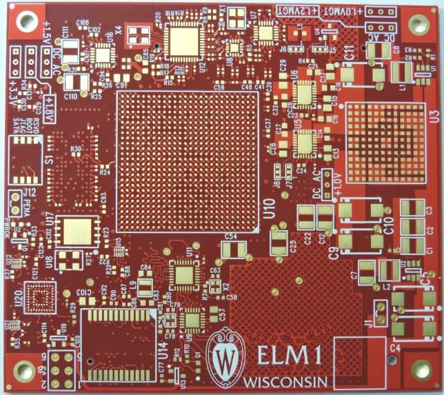
2
3

Editors
J. Brooke, R. Cavanaugh

Contributors
D. Acosta, A. Attikis, M. Bachtis, J. Berryhill, C. Botta, C. Carrillo, M. Cepeda, Y. Chen, D. Cieri,
S. Dasu, P. Dauncey, S. Dildick, C. Foudas, B. Gomber, T. Gorski, L. Guiducci, K. Hahn, P. Harris,
T. Huang, G. Iles, M. Jeitler, G. Karapostoli, M. Konecki, B. Kreis, A. Madorsky, N. Marinelli,
D. Newbold, J. Ngadiuba, I. Ojalvo, E. Perez, G. Petrucianni, V. Rekovic, T. Ruggles, P. Rumerio,
A. Safonov, A. Savin, S. Sevova, N. Smith, W.H. Smith, K. Sung, A. Svetek, A. Tapper, A. Thea,
N. Tran, M. Vicente, P. Wittich.

Acknowledgements
Feedback from all readers, the Phase-2 Upgrade coordinators, and the chair of the CMS Phase-2
TDRs editorial board (C. Lourenço) helped improve the quality of this document.
4

Contents 5
Contents
1 Introduction 7
2 Trigger Primitive Definitions and Generation 9
2.1 Tracker . . . . . . . . . . . . . . . . . . . . . . . . . . . . . . . . . . . . . . . . . . . 9
2.2 Electromagnetic Barrel Calorimeter . . . . . . . . . . . . . . . . . . . . . . . . . . 11
2.3 Hadron Barrel and Forward Calorimeters . . . . . . . . . . . . . . . . . . . . . . . 11
2.4 High Granularity Endcap Calorimeter . . . . . . . . . . . . . . . . . . . . . . . . . 12
2.5 Muon Barrel . . . . . . . . . . . . . . . . . . . . . . . . . . . . . . . . . . . . . . . . 14
2.6 Muon Endcap . . . . . . . . . . . . . . . . . . . . . . . . . . . . . . . . . . . . . . . 15
2.7 Other Triggers . . . . . . . . . . . . . . . . . . . . . . . . . . . . . . . . . . . . . . . 15
2.8 Summary . . . . . . . . . . . . . . . . . . . . . . . . . . . . . . . . . . . . . . . . . 16
3 Trigger Algorithms 17
3.1 Summary of Algorithms Previously Studied for Phase-2 . . . . . . . . . . . . . . 17
3.2 Updates to Vertex Reconstruction . . . . . . . . . . . . . . . . . . . . . . . . . . . 18
3.3 Updates to Muon Algorithms . . . . . . . . . . . . . . . . . . . . . . . . . . . . . . 20
3.3.1 Standalone Algorithms . . . . . . . . . . . . . . . . . . . . . . . . . . . . . 20
3.3.2 Displaced Muons using a Track-match Veto . . . . . . . . . . . . . . . . . 21
3.3.3 Heavy Stable Charged Particles with RPC Timing . . . . . . . . . . . . . . 22
3.4 Updates to the Electron/Photon Algorithms . . . . . . . . . . . . . . . . . . . . . 24
3.5 Updates to Tau Algorithms . . . . . . . . . . . . . . . . . . . . . . . . . . . . . . . 25
3.6 New Trigger Objects based on Particle Flow Reconstruction . . . . . . . . . . . . 26
3.6.1 Core Particle-flow Algorithm . . . . . . . . . . . . . . . . . . . . . . . . . . 26
3.6.2 Case-study: Offline Hadron-Plus-Strips Tau Algorithm . . . . . . . . . . 28
3.7 Global Algorithms . . . . . . . . . . . . . . . . . . . . . . . . . . . . . . . . . . . . 29
3.8 Heavy Ions . . . . . . . . . . . . . . . . . . . . . . . . . . . . . . . . . . . . . . . . 29
4 Menu Performance 31
5 Architectures and Conceptual System Designs 33
5.1 Introduction . . . . . . . . . . . . . . . . . . . . . . . . . . . . . . . . . . . . . . . . 33
5.2 Barrel Calorimeter Trigger . . . . . . . . . . . . . . . . . . . . . . . . . . . . . . . . 35
5.3 Barrel Muon Track Finder . . . . . . . . . . . . . . . . . . . . . . . . . . . . . . . . 36
5.4 Endcap Muon Track Finder . . . . . . . . . . . . . . . . . . . . . . . . . . . . . . . 36
5.5 Overlap Muon Track Finder . . . . . . . . . . . . . . . . . . . . . . . . . . . . . . . 37
5.6 Correlator Trigger . . . . . . . . . . . . . . . . . . . . . . . . . . . . . . . . . . . . 37
5.6.1 Regional/Layered Architecture . . . . . . . . . . . . . . . . . . . . . . . . 38
5.6.2 Time-Multiplexed Architecture . . . . . . . . . . . . . . . . . . . . . . . . 39
5.7 Global Trigger . . . . . . . . . . . . . . . . . . . . . . . . . . . . . . . . . . . . . . . 39
5.8 Summary . . . . . . . . . . . . . . . . . . . . . . . . . . . . . . . . . . . . . . . . . 39
6 Research and Development 41
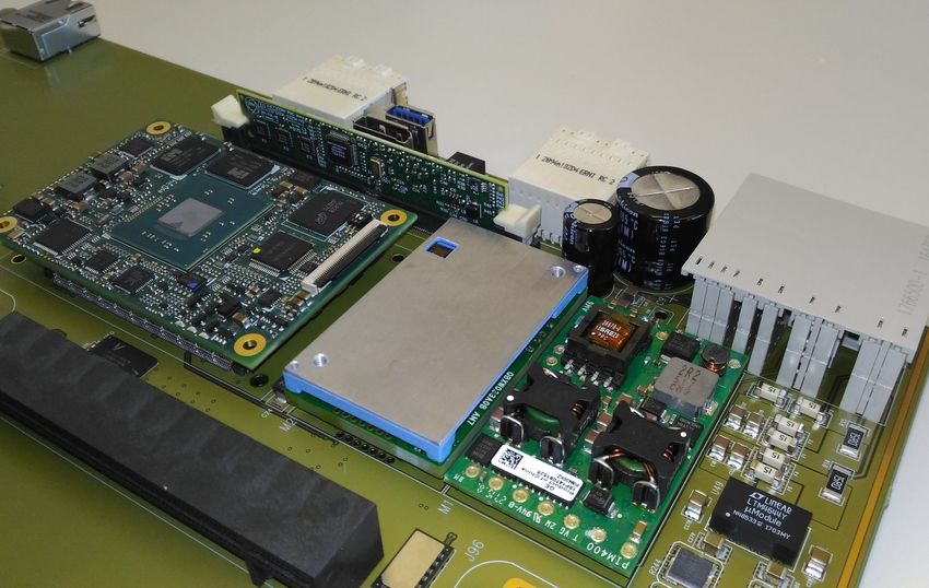
6.1 Advanced Processor Demonstrators . . . . . . . . . . . . . . . . . . . . . . . . . . 41
6                                                                                                                                           Contents

    6.2   Form Factor and Cooling . . . . . . . . .         .   .   .   .   .   .   .   .   .   .   .   .   .   .   .   .   .   .   .   .   .   .   .   42
    6.3   Configuration and Control Infrastructure          .   .   .   .   .   .   .   .   .   .   .   .   .   .   .   .   .   .   .   .   .   .   .   42
    6.4   Links . . . . . . . . . . . . . . . . . . . . .   .   .   .   .   .   .   .   .   .   .   .   .   .   .   .   .   .   .   .   .   .   .   .   43
    6.5   Memory . . . . . . . . . . . . . . . . . . .      .   .   .   .   .   .   .   .   .   .   .   .   .   .   .   .   .   .   .   .   .   .   .   44
    6.6   Firmware . . . . . . . . . . . . . . . . . .      .   .   .   .   .   .   .   .   .   .   .   .   .   .   .   .   .   .   .   .   .   .   .   44
          6.6.1  Management and Build Systems .             .   .   .   .   .   .   .   .   .   .   .   .   .   .   .   .   .   .   .   .   .   .   .   45
          6.6.2  High Level Synthesis . . . . . . .         .   .   .   .   .   .   .   .   .   .   .   .   .   .   .   .   .   .   .   .   .   .   .   45
    6.7   System Level Considerations . . . . . . .         .   .   .   .   .   .   .   .   .   .   .   .   .   .   .   .   .   .   .   .   .   .   .   46

7   Project Planning                                                                                                                                    49
    7.1 Estimated Overall Schedule . . . . . . . . . . . . . . . . . . . . . . . . . . . . . . .                                                        49
    7.2 Estimated Cost . . . . . . . . . . . . . . . . . . . . . . . . . . . . . . . . . . . . . .                                                      51

8   Appendix 1 : Trigger Primitive Word Definitions                                                                                                     53

9   Appendix 2 : List of institutions                                                                                                                   57

10 Appendix 3: Glossary of Special Terms and Acronyms                                                                                                   59

References                                                                                                                                              65
Chapter 1

Introduction

This Interim Report briefly documents the current and planned research and development that
will lead to the Phase-2 upgrade of the CMS Level-1 (L1) trigger. As such, this document
represents a roadmap to the preparation of a future Technical Design Report (TDR). Taking full
advantage of advances in Field Programmable Gate Array (FPGA) and optical link technologies
as well as their maturation expected over the coming years, the TDR for the Phase-2 upgrade
of the CMS L1 trigger is scheduled to be delivered in approximately two years from the time
of this writing. The purpose of this document is thus to complement the detector TDRs and to
provide an updated cost estimate.
The High-Luminosity LHC (HL-LHC) will open an unprecedented window on the weak-scale
nature of the universe, providing high-precision measurements of the standard model (SM)
electroweak interaction, including properties of the Higgs Boson, as well as searches for new
physics beyond the standard model (BSM) involving weak-scale couplings, such as possible
explanations for the observed gauge hierarchy or the quantum nature of dark matter. Such
precision measurements and searches require information-rich datasets with a statistical power
that matches the high luminosity provided by the Phase-2 upgrade of the LHC. Efficiently
collecting those datasets will be a challenging task, given the harsh pileup environment of 200
proton-proton interactions per LHC bunch crossing.
The CMS trigger currently comprises two levels [1]. The L1 trigger consists of custom hard-
ware processors that receive data from calorimeter and muon systems, generating a trigger
signal within 3 µs, with a maximum rate of 100 kHz. The full detector is read out on receipt
of a Level-1 Accept (L1A) signal, and events are built. The High-Level Trigger (HLT) is imple-
mented in software and reduces the rate to ∼1 kHz. This two-level strategy will not change for
Phase-2, although the entire trigger and DAQ system will be replaced. The detector readout
electronics and DAQ will be upgraded to allow a maximum L1A rate of 750 kHz, and a latency
of 12.5 µs (or 500 LHC bunch crossings). In addition, the L1 trigger will, for the first time,
include tracking information and high-granularity calorimeter information. For planning pur-
poses, and throughout this document, we target a maximum rate of 500 kHz, and a maximum
latency of 9.5 µs, with the remainders kept as contingency.
At the highest level, the L1 trigger can be divided into subsystems shown in Fig. 1.1. The Outer
Tracker will provide tracks via a Track Finder (TF) Trigger Primitive Generator (TPG) to the L1
trigger and will be key for keeping trigger thresholds and efficiencies consistent with LHC Run
1 values. An Endcap Calorimeter TPG (ECT) and a Barrel Calorimeter Trigger (BCT) system
will process the high-granularity readout of the CMS calorimetry, producing high-resolution
clusters for later processing. Endcap and Barrel Muon Track Finding (EMTF and BMTF) Trigger
systems will incorporate additional chambers covering pseudorapidity up to |η | < 2.5 and
apply state-of-the-art algorithms to efficiently identify muons. A new Correlator Trigger (CT)

                                               7
8 Chapter 1. Introduction
system will match tracks with the Calorimeter and Muon Trigger information, apply intricate
object identification algorithms, and provide a list of sorted trigger objects to a Global Trigger.
Finally, the Global Trigger (GT) will process significantly more information than the current
system, and apply much more sophisticated algorithms, in order to produce an L1A. This is
sent to the CMS Trigger Control and Distribution System (TCDS) [2], which distributes it to the
subdetector backend electronics, initiating readout to the data acquisition system (DAQ). The
latency targets for each processing step are given in Table 1.1.
TRK EC EB HB HF DT RPC CSC GEM
EB HB HF BM RPC CSC GEM
TPG TPG TPG TPG TPG TPG TPG
Track Endcap Barrel Endcap
Barrel
Finder Calo Muon Muon
Calo
TPG TPG Track Track
Trigger
Finder Finder
Correlator Trigger
CT-
PPS
possible direct links from TF
Global
possible direct links to GT BPTX
Trigger
L1 Trigger Project BRIL
Figure 1.1: High-level view of the Phase-2 L1 trigger. The main data flow is shown with solid
lines. Additional data paths are under study, including direct connections from systems up-
stream of the Correlator Trigger to the Global Trigger, and paths that allow Tracker data to be
passed to the Muon Triggers. Shown in the diagram are the Outer Tracking Detector (TRK), the
Endcap Calorimeter (EC) System, the ECAL Barrel (EB), the HCAL Barrel (HB), the HCAL For-
ward Detector (HF), the Muon Drift Tube Detectors (DT), the Resistive Plate Chambers (RPC),
the Cathode Strip Chambers (CSC), the Gas Electron Multiplier Chambers (GEM). Shown also
are the TOTEM precision proton spectrometer (CT-PPS), Beam Position and Timing Monitors
(BPTX), and luminosity and beam monitoring detectors (BRIL).
Table 1.1: Targets for L1 trigger data processing latency, indicated by absolute time after the
collision.
Processing step Time (µs)
Input data received by CT 5
Trigger objects received by GT 7.5
L1A received by TCDS 8.5
L1A received by front-ends 9.5Chapter 2
Trigger Primitive Definitions and Generation
In this chapter, we summarize the input to the Phase-2 L1 trigger, namely the Trigger Primi-
tives (TPs), that are generated in the subdetector back-end electronics. For Runs 1 and 2, the
TPs comprised tower energy sums from the electromagnetic (ECAL) and hadron calorimeters
(HCAL), track stubs from the drift tube (DT) and cathode strip chambers (CSC), and hits from
the resistive plate chambers (RPC). For Phase-2, the addition of central tracking information en-
ables the use of the full detector information, resulting in substantial improvements in trigger
performance. The new endcap calorimeter will identify energy clusters with excellent spatial
resolution and send them to the L1 trigger. In addition, upgrades of the ECAL, HCAL, and DT
back-end electronics will enable the use of high-speed optical links and therefore finer grained
information can be sent to L1. Spare input capacity will be reserved, to facilitate potential fu-
ture upgrades, for example the addition of information from the pixel detector and/or a fast
timing detector.
In the sections below, we describe the objects that form the logical interface between the sub-
detectors and the L1 trigger system. The algorithms and hardware that generate these objects
are (or will be) described in detail in the subdetector TDRs, but are also summarized below for
completeness. In most cases, the number of trigger primitive objects that are sent to L1 is fixed
by the detector geometry. However, the number of tracks, stubs, and clusters will vary from
event to event, and high occupancy events may exceed the bandwidth available. We cater for
sufficient input bandwidth that the probability for this occurence will be less than 10−4 . As-
suming such events are flagged and automatically accepted, this corresponds to a trigger rate
of only ∼3 kHz.
2.1 Tracker
A major new functionality of the CMS detector for the HL-LHC is the inclusion of data from
the Outer Tracker in the L1 trigger, facilitated by the readout of silicon tracking information at
an unprecedented 40 MHz data rate. The primary function that enables this improvement is
the ability to perform local transverse momentum (pT ) measurements with the detector front-
end electronics. Although the raw data rate generated by the sensors is enormous, most tracks
produced in LHC collisions have a very soft pT . Studies have shown [3] that 97% (99%) of the
particles created in pp interactions at 14 TeV have pT < 2 GeV (pT < 3 GeV). The readout rate
of soft interactions can be reduced by a factor of 10 via selections on the local pT measurements.
The local pT measurement is made possible by the pT module concept [4]. Pairs of closely
spaced detector layers are inspected to see if they have pairs of clusters consistent with the
passage of a high momentum particle. For each hit in the inner layer (closer to the interaction
point), a window is opened on the outer layer. If a hit is found within the window, a stub is
910 Chapter 2. Trigger Primitive Definitions and Generation
CMS Phase-2 Simulation, = 200, Minbias
Entries [a.u.]
2 GeV with truncation
2 GeV w/o truncation
3 GeV with truncation
3 GeV w/o truncation
NTracks
Figure 2.1: Number of tracks found by the track finder, for two pT thresholds, in simulated
minimum-bias collision events at 200 pileup. The effect of event truncation at the stub-level
(events with sufficiently high occupancy that not all stubs can be received) is shown by the
points, while the dotted line shows the distribution without this effect.
generated. Each stub consists of a position and a rough pT measurement. Modules comprising
of two layers of strip detectors are used in the three outer layers of the barrel and the outer
radial region of the forward disks, while modules comprising of one strip layer and one pixel
layer are used in the three inner layers of the barrel and the inner radial region of the forward
disks.
The addition of tracking information yields numerous improvements in trigger performance,
that will be discussed further in Chapter 3. In nearly all cases, to realise such improvements,
full track reconstruction is required. At pileup of 200, around 15 000 stubs will be sent from
the detector to the Track Finder (TF) TPG, also refered to as the Track Trigger in some cases,
located in an underground counting room, known as USC55. The TF must reconstruct tracks
with high efficiency, within approximately 5 µs, including 1 µs for data transmission from the
detector. Track reconstruction under these constraints represents a significant challenge. CMS
has therefore pursued three different approaches to a solution: one using associative memory
ASICs in conjunction with FPGAs, and two based exclusively on FPGAs. Hardware demon-
strators have been constructed for each approach, the results of which are described in more
detail elsewhere [4].
Regardless of the TF architecture, an average of about 200 tracks will be sent to the L1 trigger
per bunch crossing at 200 pileup. We estimate that 100 bits per track are sufficient to encode
the track parameters with no degradation in performance; a preliminary word assignment is
given in Table 8.1. The bandwidth between the TF and the L1 trigger must be sufficient to avoid
truncation of tracks in of busy events, or regions with high track density. As shown in Fig. 2.1,
to keep the probability of event truncation at the track-level below 10−4 , capacity for at least
400 tracks is required. Note that Fig. 2.1 also shows the effect of event truncation at the stub-
level (events with sufficiently high occupancy so that not all stubs can be received by the TF),
which is different from event truncation at the track-level (events with sufficiently high track
multiplicity so that not all tracks can be transmitted to the Level-1 trigger). Detailed studies
will be performed once the TF architecture is finalised, to ensure truncation effects can be kept2.2. Electromagnetic Barrel Calorimeter 11 to a similar level. Finally, we anticipate that the number of fibres will be driven by the number of TF processor cards. For the purpose of this document we assume 150 TF processor cards, each of which sends two 16 Gb/s fibres to the L1 trigger. 2.2 Electromagnetic Barrel Calorimeter To meet the increased trigger latency and rate requirements of CMS at the HL-LHC, the ECAL barrel trigger and readout electronics will be upgraded. For Phase-1, the ECAL barrel trigger primitive generator (EB TPG) is located on-detector, and produces trigger tower sums of 5 × 5 crystals. For Phase-2, the EB TPG will be entirely located in the back-end electronics, receiv- ing crystal data that will be sent from the detector. Two options for EB trigger primitive (TP) words are being investigated: a baseline single crystal primitive word, and an optional cluster primitive word. In both cases, the EB TPG must include calibration of the input data, as well as digital filtering of input pulses to extract the transverse energy (ET ) and time information. Because of mechanical constraints, each front-end card will collect data from a 5 × 5 array of crystals at 160 MHz sampling frequency. Twelve such cards will send data to a single back end card, via 48 upstream links and 12 downstream links. Each back-end card covers a region of 300 crystals equivalent to η × φ = 0.26 × 0.35. A total of 108 back-end cards, housed in 9 crates, cover the full ECAL barrel. Each crate receives data from a φ sector of the detector, and both positive and negative η. This architecture allows for sharing boundary data between regions of the detector connected to the same back-end card, which is required if clusters are sent to the L1 trigger, and also identification of “spikes” (anomalous signals resulting from charged particles incident on the ECAL photodetectors) [5]. The baseline EB TP is a 16 bit word for each of the 61 200 crystals that encodes ET , time, and a spike flag bit, summarized in Table 8.2. The data will be sent across a total of 3060 optical fibres, corresponding to 90 back-end cards with thirty 16 Gb/s links and 18 back-end cards with twenty 16 Gb/s links. Studies of cluster primitive words, generated directly in the EB TPG, are ongoing as a possible future option. Such a capability, even if limited, could prove useful later if processing within, or bandwidth into, the L1 trigger becomes constrained. For illustrative purposes, an example 40-bit word is defined to encode ET , time, and spike flags, as well as η and φ coordinates for the cluster maximum, is given in Table 8.3. Figure 2.2 shows the multiplicity distributions of ECAL offline clusters in simulated events with 200 pileup. The offline clusters shown here are taken as a proxy for a future TP cluster, and the result will need to be re-confirmed with a realistic TP algorithm. We currently assume that a capacity to transmit of order 1000 clusters per bunch crossing will be required to limit truncation effects to 10−4 . In such a case, a 16-bit word that sums the crystal energy within a region of 25 × 25 crystals would also be sent to the L1 trigger to account for any unclustered energy. 2.3 Hadron Barrel and Forward Calorimeters The Phase-2 upgrade of the HCAL Barrel (HB) calorimeter replaces the back-end electronics, and partially replaces a few front layer scintillator tiles [5] if warranted by the level of radiation damage predicted to occur during the HL-LHC. The number of readout channels, the trans- verse (η − φ) segmentation, and number of longitudinal readout depths of the HB will remain as after the Phase-1 upgrade, which is scheduled for completion during LS2. The Phase-2 HB TPG electronics will use the same hardware that is being developed for the EB,
12                                                             Chapter 2. Trigger Primitive Definitions and Generation

                                             CMS      Phase-2
                                             CMS Simulation, s = 14 Simulation,
                                                                    TeV, PU=200  = 200, Minbias

                   Entries [a.u.]
                             Nev
                                         3                                            ET >0.2 GeV
                                    10
                                                                                      ET >0.5 GeV
                                                                                      ET >1 GeV
                                                                                      ET >2 GeV
                                    10 2                                              ET >3 GeV

                                     10

                                         1

                                             0   100   200   300   400   500   600   700     800    900   1000
                                                                                                        NBC
                                                                                           NEM-Barrel-Clusters

Figure 2.2: Number of ECAL offline clusters found above a range of thresholds in simulated
events at 200 pileup.

to optimize development, production, operations and maintenance resources. For each of the
2304 trigger towers, signals from four depth segments (or three for towers with the highest η)
will be sampled at 40 MHz and corrected for pedestal, gain and response. The depth samples
for each tower are then summed and a peak detection algorithm is applied. In addition to the
tower ET , the HB TP comprises several feature bits that will facilitate encoding of longitudinal
shower profile data, for use in calibration, lepton isolation, and identification of minimum-
ionizing particles (MIPs). The baseline TP is summarized in Table 8.4.
The HF detector will continue to operate with the Phase-1 front-end and back-end electronics.
In its current configuration, the HF back-end electronics cannot sustain the L1A rate foreseen
for Phase-2. This limitation will be overcome by re-using the Phase-1 HB and HE back-end
cards, made available by the Phase-2 upgrades, to augment the existing HF back-end. The HF
TP definition will remain as in Phase-1. Signals from long and short fibres in each tower, sam-
pled at 40 MHz, are used to determine the tower energy, along with a time measurement from
a time-to-digital converter (TDC). The ET reconstruction algorithm includes suppression of the
collision-induced anomalous signals that arise when charged particles interact directly with the
photomultiplier tube windows. Two feature bits are available for each HF TP. One is used to
indicate that the ratio of the energy measured in the long versus short fibres is consistent with
the deposit of an electromagnetic shower, while the other is an ADC-over-threshold indicator
with individual thresholds per channel to define minimum-bias triggers. The number of links
used to transmit the HF TP to the L1 trigger will remain unchanged with respect to Phase-1.

2.4    High Granularity Endcap Calorimeter
The Phase-2 endcap calorimeter (EC) will be an entirely new high granularity sampling cal-
orimeter, using silicon and scintillator as the sensitive elements. Each endcap will have 52
sensitive layers, with 28 in the electromagnetic section and the remaining 24 in the hadronic
section. All the latter will contribute data to the trigger, but because of financial constraints
only half of the electromagnetic section layers will be used.
The main raw trigger data from the calorimeter will be “trigger cells”, which are sums of in-
dividual channels. The trigger cells will have an area of approximately 4 cm2 in the silicon
2.4. High Granularity Endcap Calorimeter 13 regions, with larger cells used in the scintillator region. The bandwidth to read out all trigger cells would be prohibitive, so a selection in the front-end electronics will be made with a nomi- nal threshold in ET corresponding to the energy of 2 MIP deposits (multiplied by the trigger cell sin θ). This corresponds approximately to a 10 MIP cut at the inner edge and a 4 MIP cut at the outer edge. To compensate for the resulting loss of energy, the channels will also be summed over larger areas, such that they can be read out within a reasonable bandwidth without any suppression being required. These values will be used to form a “tower map” of transverse energy on an η, φ grid. The Endcap Calorimeter TPG (ECT) will be described in detail in the EC TDR, in preparation at the time of this writing. A brief description of the ECT is presented here. The ECT data is processed in two stages. The first stage will consider each layer separately, forming two- dimensional (2D) clusters from trigger cells, and summing tower data into a single η, φ grid for the particular layer being processed. The second stage will then combine the 2D clusters in depth to form three-dimensional (3D) clusters. It will also combine all the single-layer tower map data with an appropriate weighting into the complete transverse energy tower map. We envisage using time-multiplexing to transfer all the 2D clusters and tower maps for a single bunch crossing into one FPGA. A time multiplexing period of 18 or 24 would be sufficient for this purpose. Preliminary studies of the firmware implementation indicate that trigger primitive generation within 5 µs of the bunch crossing is feasible in this architecture, including the time (up to 600 ns) added by the time-multiplexing. The completed tower maps and 3D clusters form the ECT primitives that are transmitted to the L1 trigger. For most of the EC, the tower map will have equal bins in the η, φ space of π/36 = 0.0873, which matches the geometry of the barrel calorimeter towers. This is required as there is some overlap in angular acceptance between the EC and the barrel calorimeter; the minimum |η | for the EC is approximately at 1.32. However, at high |η | this tower area becomes comparable with single trigger cells, so we foresee coarser towers outside the L1 tracking acceptance, i.e. |η | > 2.4, and a total of 1200 towers per endcap. The trigger primitive for each tower is assumed to comprise 16 bits; a 12-bit transverse energy value and a 4-bit electromagnetic fraction. With a least significant bit (LSB) for the transverse energy of 100 MeV, this would allow a reasonable precision of around 5% for track-energy matching of the lowest momentum tracks, and would have a full range of 400 GeV. There is a large amount of data associated with the 3D clusters which could be potentially useful in the L1T correlator for forming particle objects. It is not yet clear which of these data will prove to be most important. Table 8.5 shows a conceptual data format for the 3D clusters that contains many of the potential items. It has a fixed amount of information per cluster totalling 128 bits, and also some optional extra data values which could extend the size up to 416 bits in total. The basic information includes the transverse energy, subdetector section fractions, shower position, and general quality information like number of trigger cells and the maximum energy layer. The “extra data flags” indicate the presence of the optional data, which include cluster shape information, transverse energy interpreted for an electromagnetic shower, and subclusters, i.e. any local maxima that can be identified. The average size of the 3D clusters has not yet been determined; a value of about 200 bits per cluster is assumed to be typical here. The bandwidth required to transmit all 3D clusters is prohibitive, so a ET threshold is needed. The clusters are dominated by pileup so their transverse energy spectrum falls steeply and is very sensitive to the threshold. Since the clusters are the main EC input to the particle flow algorithm in the correlator, it seems important to retain clusters that may be matched to tracks.
14                                                               Chapter 2. Trigger Primitive Definitions and Generation

The L1 tracking threshold will be around ET of 2 or 3 GeV but with a gradual turn-on, so a 3D
cluster selection of ET > 1.0 GeV would be appropriate. Studies show that this cut results in up
to 400 clusters (200 per endcap); as illustrated in Fig. 2.3. Hence, a bandwidth of around 80 kb
per bunch crossing for the 3D cluster data will be required.

                                            CMS Phase-2
                                                 Number ofSimulation,
                                                           3D-clusters out√sof=trigger
                                                                                 14 TeV,  = 200
                                                                                       Layer-2
                   Entries [a.u.]
                              a.u.

                                                ET > 3.0 GeV
                                                                                                Minbias
                                     10−1          ET > 2.0 GeV
                                                        ET > 1.0 GeV
                                                                         ET > 0.5 GeV

                                     10−2

                                     10−3

                                     10−4

                                            0       50    100   150    200   250   300   350   400   450      500
                                                                                                           # C3d
                                                                                                N3D-Clusters
Figure 2.3: Number of 3D clusters per endcap reconstructed in simulated tt events with 200
pileup. The thresholds applied to the 3D clusters are ET = 0.5 GeV (blue), 1.0 GeV (pink),
2.0 GeV (green) and 3.0 GeV (black).

With the above assumptions, the total bandwidth (including both endcaps) to the L1T corre-
lator would be around 120 kb, requiring around 300 links running at 16 Gbit/s. The financial
implications of varying this bandwidth in either direction are small for the ECT in the current
design, as there is extra output capacity and so the only cost is in the fibre optic cables between
the ECT and the L1T correlator.

2.5    Muon Barrel
The current barrel muon trigger primitives consist of local muon stubs from the Drift Tube
(DT) chambers, and hits from the Resistive Plate Chambers (RPC) system. Both the DT trigger
primitive generator and the RPC Link Board system that supply data to the L1 trigger will be
replaced for Phase-2. The goals for the Phase-2 trigger primitive generation include maximising
efficiency from aging detectors, exploiting the full spatial resolution of the DT system, and
improving the time resolution of RPC clusters delivered to the trigger from 25 ns to 1 ns. The
trigger primitive generation for the barrel muon system will be performed in 84 processor
boards, which will be of the same type as those used for barrel muon track-finding. These
processors will receive 30.7 Tb/s/sector from the DT system and 0.3 Tb/s from the RPC system,
on 10 Gb/s links. A range of studies of DT stub identification algorithms have been performed,
and are described elsewhere [6]. These studies include the precise definition of the barrel muon
trigger primitives, though a possible data format for DT stubs is given in Table 8.6 and for RPC
clusters in Table 8.8. It is anticipated that these definitions may be agumented, by including the
position of the hits contributing to a stub, such that the final track-finding may perform fitting
with the full hit precision. While independent paths for DT and RPC trigger primitives reduce
sensitivity to detector issues, extensions to the muon barrel TPG that combine both are under
study, since this is expected to provide the optimum performance when both are available
2.6. Muon Endcap 15 with high efficiency. The possibility of receiving stubs from the Outer Tracker, via the TF, is also being explored, as this may improve efficiency for identifying muon tracks with displaced vertices. 2.6 Muon Endcap The endcap muon system currently comprises CSC and RPC detectors. By the time of HL- LHC, the coverage will have been extended by the addition of improved RPC (iRPC) and Gas Electron Multiplier (GEM) chambers. All detectors will provide TPs to the L1 trigger. The TPs for existing detectors will not change, except when combining local information across detectors, such as a GEM-CSC integrated local trigger which will deliver CSC TPs with a new data format to the muon track-finder. Although the CSC TPG electronics will be upgraded for Phase-2, the TPs will comprise track stubs, retaining the same data format used in Phase-1 (Table 8.7). Improvements to the stub reconstruction algorithm are envisaged to mitigate inefficiences that arise at high pileup. These include improved ghost (i.e. ambiguous and/or fake) track cancellation logic, reduction of pre- trigger deadtime, optimised pattern recognition, and improved timing. A total of 588 optical links operating at 3.2 Gb/s will send the CSC TPs to the L1 trigger. The existing endcap RPC detectors have only one layer and hence the trigger primitives are single hits. While the electronics will be upgraded to facilitate fast link speeds, no change is envisaged in the data format, which is given in Table 8.8. The new iRPC detectors (RE3/1 and RE4/1) will have no segmentation in η. Instead, they will be equipped with precision timing electronics to measure the η position from two timing measurements of the hit. The proposed data format for iRPC TPs is given in Table 8.9, and will be sent to the L1 Trigger on forty-eight 10 Gb/s links. The GEM detectors will provide information to the L1 trigger via two distinct paths. First, clusters are reconstructed by grouping hits in each GEM layer, and sent to the L1 trigger using the format given in Table 8.10. The GEM TPs are transmitted to the L1 trigger on 252 links operating at 10 Gb/s. In addition, clusters will be sent to the CSC TPG, and used to reconstruct integrated GEM-CSC track stubs. The integrated stub algorithm improves the local reconstruc- tion efficiency in ME1/1-GE1/1 and ME2/1-GE2/1 by 3% and 10% respectively, at pileup of 140. In areas where the CSCs might show signs of aging and be operated at lower high voltage, the GEM chambers can recover efficiency by as much as 30%. The data format of the GEM- CSC TPs, shown in Table 8.11, comprises the same number of bits as the Phase-1 CSC stub data format. For GEM ME0, the on-detector electronics will reconstruct hits and clusters. However, since ME0 will have six layers, transmitting raw clusters to the L1 trigger would require a large number of links. Instead, the ME0 TPs comprise multi-layer stubs reconstructed from clusters. The TPG algorithm will be able to measure the stub η and φ position, and direction with high precision. Although the ME0 stub data format is not defined yet, it could be very similar to the CSC data format. A possible data format is given in Table 8.12. Forty-eight 10 Gb/s links are required to transmit the TPs to the L1 trigger. 2.7 Other Triggers Several subdetectors will not provide trigger primitives, but will provide simple binary logic signals for inclusion in the trigger menu logic. These include: the Beam Position and Timing
16                                     Chapter 2. Trigger Primitive Definitions and Generation

Monitors (BPTX) that are used for zero bias triggers, the TOTEM precision proton spectrometer
(CT-PPS), and other luminosity and beam monitoring detectors. These signals will be received
directly by the Global Trigger, via a custom interface board.

2.8     Summary
The logical TP inputs to the Phase-2 L1 trigger are summarized in Table 2.1.

             Table 2.1: Summary of the logical input data to the Phase-2 L1 trigger.
      Detector     Object N bits/object N objects N bits/BX Required BW (Gb/s)
      TRK           Track       100             400        40 000             1 600
      EB           Crystal       16           61 200      979 200            39 168
      HB           Tower         16            2 304       36 864             1 475
      HF           Tower         10            1 440       13 824              553
      EC           Cluster      200             400        80 000             3 200
      EC           Tower         16            2 400       38 400             1 536
      MB DT         Stub         70             240        33 600             1 344
      MB RPC       Cluster       15            3 200       48 000             1 902
      ME CSC        Stub         32            1 080       34 560             1 382
      ME RPC       Cluster       15            2 304       34 560             1 382
      ME iRPC      Cluster       41             288        11 808              472
      ME GEM       Cluster       14            2 304       32 256             1 290
      ME0 GEM       Stub         24             288        6 912               276
      Total           -           -              -            -              53 980
Chapter 3
Trigger Algorithms
Maintaining trigger thresholds that are similar to Phase-1 of the LHC during the harsh, high-
luminosity running conditions of the Phase-2 LHC will be of paramount importance for effi-
ciently collecting statistically powerful datasets at electroweak mass scales. To achieve man-
ageable data recording rates, it will be crucial to identify the primary event interaction vertex
and to mitigate pileup effects from 200 hundred other proton interactions that take place ev-
ery LHC bunch crossing. Furthermore, it is important to match the performance of algorithms
running in the online trigger with the corresponding algorithms running in the offline recon-
struction, which make extensive use of tracking information: well-matched algorithms provide
a sharpened “turn-on” of the efficiencies that reduce rates and enable lower thresholds. For
these reasons, a track finder TPG [4] will be key in providing tracking information for object
algorithms running in the hardware of the L1 trigger.
The R&D strategy employed here develops three classes of trigger algorithms: (1) standalone
objects, (2) track-matched objects, and (3) particle-flow objects. Standalone trigger algorithms
represent an important part of the Phase-2 trigger menu, since they provide a robust ability to
trigger using independent subdetectors; they also provide a reference upon which to compare
improvements from more sophisticated algorithms that combine information across detectors.
Track-matched algorithms, which use tracking to confirm standalone calorimeter objects, are
expected to provide significant performance improvements with respect to just standalone cal-
orimeter algorithms, while maintaining relative simplicity in their design. Finally, particle-flow
algorithms are expected to provide the ultimate performance improvement, as they combine in-
formation optimally and best match the offline algorithms; they also require the most process-
ing time and resources to complete their calculations. The complete suite of Phase-2 triggers
available for the trigger menu is therefore expected to be rich and the processing performed by
the upgraded L1 trigger must support a diverse set of requirements.
As the Phase-2 upgrade of the L1 trigger progresses through the current R&D period, from
conceptual to final design, a complete list of core trigger algorithms will be developed and
studied. Much of the groundwork to develop and study algorithms that match track-trigger
information with standalone calorimeter or muon trigger objects has already been performed
and reported elsewhere [3]. We summarize those findings below. Only updates to those algo-
rithms or additional examples of algorithms that further illustrate the potential of the Phase-2
upgrade of the L1 trigger are detailed in this interim report.
3.1 Summary of Algorithms Previously Studied for Phase-2
Early studies presented in Ref. [3] applied a prototype TF using full simulations of the Phase-1
CMS detector to develop standalone trigger objects matched to tracks above a pT threshold
1718 Chapter 3. Trigger Algorithms of 2 GeV. Those studies conclusively demonstrate both the benefit of and the need for such algorithms to efficiently trigger the readout of the CMS detector at the HL-LHC. Both inside-out and outside-in algorithms that match muons to tracks were studied and shown to provide similar performance. Very good efficiency (greater than 95% on the trigger plateau) is observed and a rate reduction factor of between 6 and 10 is achieved for a non-isolated muon pT threshold of 20 GeV, due to the improved pT resolution from the matched track. Because of bremsstrahlung radiation losses by electrons in the outer tracker, an algorithm with two work- ing points that match electromagnetic clusters with tracks was investigated: one optimised for high pT and one optimised for low pT involving looser track quality requirements. The non- isolated, track-matched electron algorithm working points provide an efficiency that is lower than standalone calorimeter e/γ objects, but still acceptable, reaching about 95% in the barrel region, and achieve a rate reduction factor of about 6 for an electron pT threshold of 20 GeV. A track-based algorithm for determining the relative isolation of leptons was studied. The algo- rithm only considers tracks consistent with the vertex of the lepton and achieves a further rate reduction factor of somewhat less than about 2, for a total reduction factor of about 10 for track- matched electrons having pT > 20 GeV. A track-based algorithm for identifying isolated pho- tons was developed using an isolation annulus, to account for photon conversions. Rates for a double-photon trigger having pT thresholds of 18 GeV and 10 GeV are reduced by more than a factor of 6, while maintaining 95% efficiency. Two different trigger algorithms were developed for isolated tau identification, one seeded by calorimeter information and confirmed by track information, and the other seeded by both track information and electromagnetic calorimeter information. Both algorithms show comparable performance with either able to reduce the rate by a factor of about 3, while maintaining the rate and efficiency for a H → ττ signal. A fast reconstruction algorithm of the primary event vertex was developed by histogramming the z0 position of all tracks, weighted by their pT . The primary vertex position can be identified with sub-millimetre resolution and about 90% efficiency for tt̄ events with high track multi- plicities. An algorithm that matches standalone calorimeter jets to tracks was developed and is able determine the z position of the jet vertex with 95% efficiency and millimeter-level accu- racy. Multijet triggers were studied by requiring that track-matched jets share a common vertex position within 1 cm. Missing pT and scalar-summed pT triggers based on track-matched jets (HTmiss and HT ) triggers were then studied with average corrections due to pileup, providing rate reductions by factors between 5 and 10 for the examples considered in [3]. A standalone missing transverse momentum algorithm based solely on tracks within 1 cm of the identified primary event vertex was developed. This track-based MET algorithm is much more robust with respect to pileup effects and can provide up to a factor of 100 reduction in trigger rate with 90% efficiency for signals involving MET of more than 250 GeV like the examples consid- ered in [3]. Some of the algorithms summarized above have been updated using full simulations of a Phase-2 CMS detector, including the trigger primitives described in Chapter 2. Those updates, as well as new algorithms based on particle-flow reconstruction, are detailed in the following sections of this report. 3.2 Updates to Vertex Reconstruction With the availability of L1 track information, it is possible to reconstruct primary vertices in the collision at L1. This is crucially important to reject pileup in high-luminosity LHC running con- ditions. Four different algorithms have been tested, three hierarchical clustering algorithms [7] and a density-based algorithm, which have been compared with the histogramming algorithm
3.2. Updates to Vertex Reconstruction                                                                                                                                                            19

described in the CMS Phase-2 Technical Proposal [3]. This study uses updated simulations that
incorporate a new tilted geometry for the Phase-2 Outer Tracker as described in Ref. [4].

                                           CMS Phase-2 Simulation, top-quark pairs                                                       CMS Phase-2 Simulation, DBSCAN,  = 200
                                       1

                                                                                                    Vertex reconstruction efficiency
  Vertex reconstruction efficiency

                                     0.9                                                                                               0.9

                                     0.8                                                                                               0.8

                                     0.7                                                                                               0.7

                                     0.6                                                                                               0.6
                                                      DBSCAN  = 0       TP  = 0

                                     0.5                                                                                               0.5
                                                      DBSCAN  = 140     TP  = 140
                                     0.4                                                                                               0.4
                                                                                                                                                            tt
                                     0.3                                                                                               0.3
                                                      DBSCAN  = 200     TP  = 200                                                                   Charged Higgs (mh± = 500 GeV)
                                     0.2                                                                                               0.2
                                                                                                                                                            h → ZZ → 4l
                                     0.1                                                                                               0.1
                                                                                                                                                            h → ττ
                                      0                                                                                                 0
                                      −15       −10        −5           0    5            10   15                                        −15    −10    −5              0    5       10      15
                                                                            True vertex z0 [cm]                                                                            True vertex z0 [cm]

                                                                    (a)                                                                                          (b)
Figure 3.1: Efficiency for reconstructing the hard interaction primary vertex within 1.5 mm
of the true vertex, as a function of the true longitudinal impact parameter z0 . (Left) the effi-
ciency for tt̄ events with different pileup contents. (Right) the efficiency for different signals
(tt̄, H± , H → ZZ → 4l and H → ττ) with a pileup of 200.

The tracking performance of the new tilted geometry is largely unchanged or improved com-
pared with the studies presented in [3], except for the z0 resolution, which is known to be
slightly degraded due to simple geometric considerations. The L1 tracks used to find the pri-
mary vertex must have stubs in at least four different tracker layers, a transverse momentum
above a predefined threshold, and a track fit χ2 per degree of freedom of less than 20.
The density-based spatial clustering of applications with noise (DBSCAN) [8] algorithm has
been found to be the best compromise between performance and feasibility for an implemen-
tation in hardware. It shows good vertex reconstruction efficiency, excellent tolerance for noise
(i.e. fake) tracks, does not require any pre-sorting of the tracks and, most importantly, has
been already implemented on FPGA hardware [9]. For this interim report, the algorithm was
studied in software and implemented for one dimension, the estimated longitudinal impact
parameter z0 of the L1 tracks. Figure 3.1a shows the distribution of the hard interaction pri-
mary vertex reconstruction efficiency for the DBSCAN algorithm, compared with the results
obtained using the Technical Proposal histogramming method [3], as a function of the z0 posi-
tion of the true vertex in inclusive tt̄ events with different pileup content. For this study only L1
tracks with pT > 3 GeV were considered; reducing the threshold to p T > 2 GeV did not show
significant improvements. The average efficiency to reconstruct the hard interaction primary
vertex within 1.5 mm of the true vertex in tt̄ events with 200 pileup is approximately 86% using
the DBSCAN algorithm and 84% with the histogramming approach. The longitudinal impact
parameter is observed to have a resolution of σz0 = 0.49 mm.
While the DBSCAN algorithm correctly identifies the primary vertex for events with a high
multiplicity of high-pT tracks, it underperforms in events with a low multiplicity of high-pT
tracks. Figure 3.1b shows the efficiency of reconstructing the primary vertex to within 1.5 mm
for various signals superimposed on a pileup of 200 minimum-bias collisions per LHC bunch
crossing. We note that lepton and photon trigger paths would not typically require a primary-
vertex constraint. Hence, signal processes triggered by leptons or photons would not be af-
fected by the inefficiencies to reconstruct the primary vertex in such low track-multiplicity
20 Chapter 3. Trigger Algorithms events. 3.3 Updates to Muon Algorithms The present muon reconstruction and identificaton in the offline CMS software is performed by propagating the trajectory within a muon detector while taking into account the variation of the magnetic field, energy loss, and multiple scattering, using an iterative approach known as a Kalman filter [10]. For prompt muons, defined to be muons arising from the hard-scatter of the event, a vertex constraint is also applied, exploiting the additional lever-arm to improve the curvature resolution. Muons are also matched to tracks (or stubs) from the inner tracker and the more precise momentum measurement of the tracker is used for the muon momentum assignment. Within the context of the L1 trigger, good transverse momentum resolution is crucial for rate reduction, since poor resolution low momentum muons and punch-through hadrons (or their products) are more likely than good resolution muons to migrate to higher momenta and eventually pass a given momentum threshold. The current (Phase-1) muon-track finder trigger algorithms are standalone, based on simple pattern recognition solely within the Muon Detector system, and have a latency that ranges be- tween 6 and 12 BX when implemented on a Xilinx Virtex-7 FPGA. The future (Phase-2) L1 trig- ger will have tracking information available from the CMS inner tracker and the corresponding muon L1 trigger algorithms are envisaged to be done in three steps: (1) find standalone muons, built from stubs in the muon detectors; (2) match L1 tracks to standalone muons, using the more precise momentum measurement of the tracker; (3) isolate muons using L1 tracks. The anticipated gains in FPGA processing power over the coming years provide an opportunity to introduce muon reconstruction algorithms that target performance levels closer to the High Level Trigger and offline reconstruction. 3.3.1 Standalone Algorithms A Kalman filter approach has been adapted for use in the trigger hardware, taking into ac- count the energy loss and multiple scattering in the CMS return yoke. The use of advanced FPGAs, which include a large number of digital signal processor (DSP) cores, large numbers of look-up-tables (LUTs), and can operate at high clock frequency, are essential for algorithms based on a Kalman filter, because filtering is a sequential process and sufficient logic resources as well as high clock speeds are needed to keep the algorithm latency at a manageable level. The algorithm uses stubs as inputs from the muon detectors. The information of a stub consists of the station number (ρ), the azimuthal angle (φ), and the bending angle (φb ). Each track is described by the track position (φ), the track direction (φb ), and the signed curvature K = q/pT . Figure 3.2 shows the improvement in curvature resolution for the Kalman filter compared with the Phase-1 muon trigger algorithm in the CMS barrel region for two single muon samples consisting of muons with transverse momenta of 7 GeV and 100 GeV. Both the propagation and the Kalman filter update involve many mathematical operations, including a 2 × 2 matrix inversion in the update logic. Those complex calculations are approximated by performing a lookup of the Kalman gain, which was found to depend only on the station and hit pattern of the reconstructed track. A preliminary version of the algorithm, including seven propaga- tion steps and four update steps, has been implemented in firmware using Vivado High Level Synthesis (HLS), a software package from the Xilinx, targeting recent Xilinx Virtex Ultrascale FPGAs. Exploiting the DSP cores substantially reduces the other FPGA resources required, re- sulting in a total usage of 10% of the DSPs, 5% of the flip-flops, and 15% of the LUTs. Avoiding the use of the slower block RAM allows the operations to proceed at very high clock speeds. A
3.3. Updates to Muon Algorithms                                                                                                                     21

clock frequency of 360 MHz results in a total latency of 10 BX, while reducing the frequency to
200 MHz increases the latency to 12 BX. The simulations performed for this interim report are
encouraging and a future implementation in a hardware demonstrator is planned.

                      CMS
                     CMS    Phase-2µ Simulation,
                         Simulation, P = 7 GeV  = 0, Single muon
                                      T
                                                                                              CMS   Phase-2 Simulation,
                                                                                               CMS Simulation,             = 0, Single muon
                                                                                                               µ P = 100 GeV
                                                                                                                  T
                  0.5

                                                                            Entries [a.u.]
 Entries [a.u.]

                                                                                      a.u
           a.u

                                                                                             0.4
                                                       Phase 2 MTF
                                                       Kalman  (Kalman)                                                         Phase 2 (Kalman)
                                                                                                                                 Kalman  MTF
                                                                                         0.35
                  0.4    muon pT = 7 GeV                                                           muon pT = 100 GeV
                                                       Phase 1I (LUT)
                                                       Phase                                 0.3                                Phase
                                                                                                                                 Phase1I (LUT)
                  0.3                                                                    0.25
                                                                                             0.2
                  0.2
                                                                                         0.15
                                                                                             0.1
                  0.1
                                                                                         0.05
                   0                                                                          0
                   −3      −2      −1      0       1          2         3                     −4      −3   −2   −1     0    1     2     3     4
                                                            (K-Kgen)/Kgen                                                         (K- K ) / K
                                                         (K-KGEN)/KGEN                                                            (K-KGEN
                                                                                                                                      gen )/KGEN
                                                                                                                                              gen

Figure 3.2: Comparison of the resolution of the curvature K = q/pT for 7 GeV muons in the
barrel region (Left) and 100 GeV muons in the barrel region (Right) between the Phase-1 LUT
momentum assignment and the Kalman Filter algorithm.

In addition to the improvements to the barrel region expected from upgraded algorithms and
electronic boards, the installation of extra stations in the forward region (ME0, GEM, RPC) and
the electronics upgrade of various other components will improve the local stub reconstruction
efficiency, pT resolution, and the trigger capabilities for prompt muons in Phase 2. Especially
the forward region will be strengthened with additional information that will allow the endcap
muon trigger to maintain efficiency while keeping the rates sustainable. The key feature is the
measurement of the GEM-CSC bending angle in station 1, GE1/1-ME1/1, which will largely re-
duce the trigger rate. Moreover, the combination of GEM+CSC system provides redundancy in
stations 1 and 2, and so improves resilience to operational or aging effects of the CSC and GEM
detectors. In the difficult high-rapidity region, 2.0 < |η | < 2.4, the endcap muon trigger will
also use ME0 stubs to build tracks. The RPC detector information from RE3/1 and RE4/1 will
improve track reconstruction efficiency, especially in areas where spacers in the CSC detectors
fiducial volumes line up between ME3/1 and ME4/1.
The left plot of Fig. 3.3 shows that the inclusion of GE1/1 and GE2/1 information in the prompt
muon trigger increases the trigger efficiency in the plateau by 2% to 5% in the region 1.65 <
|η | < 2.15 at PU 200. The right plot of Fig. 3.3 shows that extra hit information from GEM can
significantly reduce the prompt muon trigger rate. In the region 2.1 < |η | < 2.4 rate reduction
is achieved by requiring an ME0 stub.

3.3.2                   Displaced Muons using a Track-match Veto
Many new-physics scenarios involve muons that are significantly displaced from the beamline
and, in those cases, tracks from the track trigger cannot be reconstructed for muons having
an impact parameter, |d xy |, beyond 1 cm. Standalone muons however can be reconstructed
up to a transverse displacement with respect to the beampipe, L xy , of ∼ 350 cm and up to an
impact parameter of ∼ 100 cm. The current standalone muon pT assignment applies a beam-
spot constraint, so that muons with a large displacement are not triggerable at any pT cut.
The prototype of the displaced muon algorithm drops the beam-spot constraint, but requires
precision measurements of the muon direction in at least two stations to measure momentum.
22 Chapter 3. Trigger Algorithms
CMS Phase-2 Simulation s = 14 TeV, = 200 CMS Phase-2 Simulation s = 14 TeV, = 200
Trigger rate [kHz]
Trigger efficiency
1
0.9 10
0.8
0.7
Trig
p > 14 GeV, 1.65 < |η| < 2.15 1
0.6 T
0.5
0.4 Trig
p > 14 GeV
T
0.3 Phase-2 (CSC+GE11+GE21+ME0) 10−1
0.2 Phase-1 (CSC+GE11) L1Mu(standalone) Performance
Phase-1 (CSC): Run-2 Trigger
Phase-1 (CSC): Run-2 trigger
0.1 Phase-1 (CSC+GE11)
Phase-2 (CSC+GE11+GE21+ME0)
0 10−2
1.6 1.7 1.8 1.9 2 2.1 2.2 2.3 2.4 2.5
0 5 10 15 20 25 30 35 40 45 50
True muon p [GeV]
T |η|
Figure 3.3: (Left) Prompt muon trigger efficiency as function of true muon pT in 1.65 < |η | <
2.15. (Right) Prompt muon trigger rate of prompt muon trigger with GE21 and ME0 in 2.0 <
|η | < 2.4.
An algorithm was developed for the barrel, using the direction measurement from the Phase-1
DT stubs, and in the endcaps using position and direction measurements of GEM, CSC, and
ME0. The endcap is substantially more challenging because of the coarseness of the CSC stub
direction and the much weaker magnetic field. Nevertheless, the direction measurement from
the CSCs alone is sufficient in the low-eta region 1.2 < |η | < 1.6. In the forward region,
1.6 < |η | < 2.4, the bending angle from GE1/1-ME1/1 or ME0-ME1/1 can be used to measure
the muon direction in Station 1. A second good measurement is obtained from the GE2/1-
ME2/1 bending angle. In both the barrel and endcap algorithms, a veto of the tracks from
the track-trigger extrapolated to the second muon station will be employed to offset the rate
increase from prompt muons or those arising from hadron decays in flight. Three different
veto working points have been defined, loose (pL1 T
track > 4 GeV), medium (pL1 track > 3 GeV)
T
and tight (pTL1 track > 2 GeV). This is highly efficient for prompt muons, which constitute the
majority of the background contributing to the trigger rate. The left plot of Fig. 3.4 shows the
trigger rate reduction factor as a function of pseudorapidity, after applying the track-veto. The
right plot of Fig. 3.4 shows that the barrel algorithm efficiency is independent of the muon
displacement; a similar result is found for the endcap.
3.3.3 Heavy Stable Charged Particles with RPC Timing
Several theoretical models, including many inspired by supersymmetry (SUSY), predict the
existence of Heavy Stable Charged Particles (HSCP). Since such particles are slow moving,
they can be identified with a time-of-flight measurement. The Phase-2 upgrade of the CMS RPC
back-end electronics, and in particular the link system, will provide hits with an improved time
resolution of ∼ 1.5 ns to the L1 trigger, facilitating dedicated HSCP algorithms. Moreover, the
new iRPC chambers will extend the acceptance to |η | < 2.4, providing similar time resolution
and better space resolution, to complement this search. The strategy to identify HSCPs consists
of a linear fit of RPC hits in space-time, which is not demanding in computing power. The
slope of the fit provides a measurement of the particle β (= v/c). The resolution in β of the L1
muon track is shown in Fig. 3.5 (Left). The efficiency of the proposed algorithm as a function
of the β of the slow moving particle is compared with the efficiency of a Phase-1 muon trigger,
currently used in CMS searches, in the right plot of Fig. 3.5. A clear improvement is observed
in efficiency for slowly moving particles in the region below β ∼ 0.5 c.3.3. Updates to Muon Algorithms 23
102
CMS Phase-2 Simulation s = 14 TeV, = 140 CMS Phase-2 Simulation √s = 14 TeV, = 140 PU
Ratio
Trigger efficiency
Loose veto 1
Medium veto
0.9
Tight veto
10 0.8
Trigger
0.7
p ≥ 10 GeV L1Mu (unconstrained)
T
0.6
1
0.5 0 < |η| < 0.9, pL1 ≥ 20 GeV
T
0.4 10 < |dxy| < 15 cm
0.3
10−1 25 < |dxy| < 30 cm
0.2
45 < |dxy| < 50 cm
0.1
10−20 0.5 1 1.5 2 2.5 0
0 5 10 15 20 25 30 35 40 45 50
|η| True muon p [GeV]
T
Figure 3.4: (Left) Barrel and endcap displaced muon trigger rate reduction factor versus pseu-
dorapidity after applying the lose (solid black squares), medium (open blue squares), and tight
(open red triangles) track-veto requirements. (Right) Efficiencies of the displaced muon algo-
rithm in the barrel for impact parameters between 10–15 cm (solid red circles), 25–30 cm (solid
green squares), and 45–50 cm (solid blue triangles).
CMS Phase-2 Simulation √s = 14 TeV, = 0 1
CMS Phase-2 Simulation √s = 14 TeV, = 0
Efficiency
Entries [a.u.]
0.9
Phase 1 - 25ns time resolution
0.25
Phase 2 - 1.5ns time resolution 0.8
0.2 0.7
0.6
0.15 0.5
0.4
0.1
0.3
0.2
0.05
0.1 Phase-2 RPC-HSCP trigger
Phase-1 Regular muon trigger (L1 Mu Open)
0 0
−3 −2 −1 0 1 2 3 0 0.2 0.4 0.6 0.8 1
(βGEN- βRPC )/ βGEN β
GEN
Figure 3.5: Resolution of the β measurement for L1 muon tracks using L1 trigger RPC hits
(Left), and efficiency for identifying HSCPs as a function of β for Phase-1 and Phase-2 L1 muon
triggers (Right).24 Chapter 3. Trigger Algorithms
3.4 Updates to the Electron/Photon Algorithms
The electron and photon trigger algorithms use information based on calorimeter (electromag-
netic and hadronic) and tracking detectors across the full fiducial acceptance of the respective
subdetectors, though only the barrel region is studied in this interim report, and are developed
here with the following guidelines. First, the spatial resolution should be as close as possible
to the offline reconstruction, with an ability to reconstruct electomagnetic clusters having pT
above just a few GeV and having an efficiency greater than 95% in the region above about
10 GeV. Both standalone calorimeter-only algorithms as well as track-matched to calorimeter
algorithms are required. The standalone-calorimeter-only algorithms provide up to 99% ef-
ficiency at the trigger plateau (especially important for high momentum objects), while the
track-matched to calorimeter algorithms reduce trigger rates with an acceptable minimal loss
of efficiency due to track reconstruction and matching to calorimeter clusters (especially im-
portant for low to moderate momentum objects).
CMS Phase-2 Simulation, = 200, Single e/γ CMS Phase-2 Simulation, = 200, MinBias
Efficiency (L1 Algo/Generated)
Rate [kHz]
1.2 Phase-1 L1EG (Tower)
104
Phase-2 L1EG (Crystal)
1
Phase-2 L1EG (Crystal + Trk) Electron
103
0.8 Phase-2 L1EG (Crystal) Photon
Phase-1 L1EG (Tower)
0.6 Phase-2 L1EG (Crystal) 102
Phase-2 L1EG (Crystal + Trk) Electron
0.4 Phase-2 L1EG (Crystal) Photon
10
0.2
0 1
−1.5 −1 −0.5 0 0.5 1 1.5 0 10 20 30 40 50 60
Gen η ET threshold [GeV]
Figure 3.6: (Left) Expected efficiency of the single electron trigger for the barrel region: calori-
meter only, calorimeter photon tuned trigger, and calorimeter matched to the track, compared
to the current trigger efficiency as a function of simulated |η | of the electrons/photons for a
trigger threshold of 20 GeV. (Right) Expected rate for minimum-bias events using the single
electron calorimeter trigger (for the barrel region only) as a function of trigger threshold.
Following the upgrade of both on-detector and off-detector electronics for the barrel calorime-
ters, the digitized response of every crystal of the barrel ECAL will provide energy measure-
ments with a granularity of (0.0175, 0.0175) in (η, φ), which is 25 times higher than the input
to the Phase-1 trigger consisting of trigger towers which had a granularity of (0.0875, 0.0875).
The much finer granularity and resulting improvement in position resolution of the electro-
magnetic trigger algorithms is critical in evaluating calorimeter isolation. The trigger algorithm
studied here for electons and photons mimics closely the one used in offline reconstruction and
physics analyses, albeit with a number of simplifications required by trigger latency consider-
ations. First, a core cluster is defined by a set of η × φ = 3 × 5 crystals around a seed crystal
having pT above 1 GeV, with a possible extension along the φ direction to take into account
bremsstrahlung energy losses. The cluster position is determined as an energy weighted sum
of the individual crystals within the cluster, and the isolation of each cluster is calculated us-
ing 27 × 27 crystals around the seed crystal. Shower shape variables from the 3 × 5 crystals
within the core cluster are then used to determine two operating points: one for electrons and
photons, and a second for photons only. HCAL information is not yet directly used to identifyYou can also read