Cushion bogs are stronger carbon dioxide net sinks than moss-dominated bogs as revealed by eddy covariance measurements on Tierra del Fuego, Argentina
←
→
Page content transcription
If your browser does not render page correctly, please read the page content below
Biogeosciences, 16, 3397–3423, 2019
https://doi.org/10.5194/bg-16-3397-2019
© Author(s) 2019. This work is distributed under
the Creative Commons Attribution 4.0 License.

Cushion bogs are stronger carbon dioxide net sinks than
moss-dominated bogs as revealed by eddy covariance
measurements on Tierra del Fuego, Argentina
David Holl1 , Verónica Pancotto2,3 , Adrian Heger1 , Sergio Jose Camargo3,4 , and Lars Kutzbach1
1 Institute
          of Soil Science, Center for Earth System Research and Sustainability (CEN),
Universität Hamburg, Hamburg, Germany
2 Centro Austral de Investigaciones Científicas (CADIC-CONICET), Ushuaia, Argentina
3 Universidad de Tierra del Fuego (ICPA-UNTDF), Ushuaia, Argentina
4 Dirección de Cambio Climático (DCC), Secretaría de Estado de Ambiente,

Desarrollo Sostenible y Cambio Climático (SADSyCC), Ushuaia, Argentina

Correspondence: David Holl (david.holl@uni-hamburg.de)

Received: 24 April 2019 – Discussion started: 8 May 2019
Revised: 2 August 2019 – Accepted: 5 August 2019 – Published: 12 September 2019

Abstract. The near-pristine bog ecosystems of Tierra del          stayed on similar levels. A higher amount of available radi-
Fuego in southernmost Patagonia have so far not been stud-        ation in the second observed year led to an increase in GPP
ied in terms of their current carbon dioxide (CO2 ) sink          (5 %) and NEE (35 %) C uptake. The average annual NEE-
strength. CO2 flux data from Southern Hemisphere peat-            C uptake of the cushion bog (−122 ± 76 g m−2 a−1 , n = 2)
lands are scarce in general. In this study, we present CO2        was more than 4 times larger than the average uptake of the
net ecosystem exchange (NEE) fluxes from two Fuegian bog          moss-dominated bog (−27 ± 28 g m−2 a−1 , n = 2).
ecosystems with contrasting vegetation communities. One
site is located in a glaciogenic valley and developed as a peat
moss-dominated raised bog, and the other site is a vascu-
lar plant-dominated cushion bog located at the coast of the       1   Introduction
Beagle Channel. We measured NEE fluxes with two identi-
cal eddy covariance (EC) setups at both sites for more than       Although peatlands cover a comparably small area of the
2 years. With the EC method, we were able to observe NEE          Earth’s land surface, they store large amounts of carbon (Yu
fluxes on an ecosystem level and at high temporal resolu-         et al., 2010). Intact peatlands act as net sinks for atmo-
tion. Using a mechanistic modeling approach, we estimated         spheric carbon (C) and play an important role in the ter-
daily NEE models to gap fill and partition the half-hourly net    restrial C cycle and therefore in the climate system. While
CO2 fluxes into components related to photosynthetic uptake       in-depth studies of long-term and recent carbon accumu-
(gross primary production, GPP) and to total ecosystem res-       lation rates are available for many Northern Hemisphere
piration (TER). We found a larger relative variability of an-     bogs, carbon flux data from Southern Hemisphere bogs are
nual NEE sums between both years at the moss-dominated            scarce. The Magellanic Moorland, which covers an area of
site. A warm and dry first year led to comparably high TER        44 000 km2 of coastal Patagonia in Chile and Argentina, is
sums. Photosynthesis was also promoted by warmer condi-           one of the most notable peatland complexes south of the
tions but less strongly than TER with respect to absolute and     Equator and belongs to the world’s largest wetlands (Fraser
relative GPP changes. The annual NEE carbon (C) uptake            and Keddy, 2005). Significant parts of the Magellanic Moor-
was more than 3 times smaller in the warm year. Close to the      land are dominated by a unique type of bog ecosystem,
sea at the cushion bog site, the mean temperature difference      which is exclusive to the Southern Hemisphere. These so-
between both observed years was less pronounced, and TER          called cushion bogs are rainwater-fed peatland ecosystems,

Published by Copernicus Publications on behalf of the European Geosciences Union.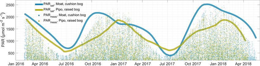
3398                                                            D. Holl et al.: Cushion bogs are strong carbon dioxide net sinks

which are dominated by the vascular plants Astelia pumila             that account, our initial objective is to comprehensively de-
(J. R. Forst.) Gaudich. (Govaerts, 2019) and Donatia fascic-          scribe the CO2 net ecosystem exchange (NEE) flux dynamics
ularis (J. R. Forst. & G. Forst.) (Ulloa Ulloa et al., 2017) as       of two contrasting bog ecosystems on Tierra del Fuego us-
opposed to the majority of global bogs, which are commonly            ing an EC setup. We apply a mechanistic modeling approach
peat moss-dominated. Both cushion plants are characterized            yielding a partitioned net CO2 flux with two model terms
by high nutrient use efficiency, slow biomass turnover and a          estimating total ecosystem respiration (TER) and gross pri-
large root biomass in relation to the small aboveground part          mary production (GPP) separately. We finally compare our
of the plants (Kleinebecker et al., 2008). Fritz et al. (2011) es-    data with literature records of Northern and Southern Hemi-
timated fine root biomass accumulation to be 4 times larger           sphere NEE balances and whole ecosystem C balances taking
in cushion bogs than in Northern Hemisphere raised bogs.              into account methane flux data that have been published for
The aerenchymatic roots of vascular cushion plants lead to            the two sites of this study.
additional oxygen transport to the rhizosphere and thereby to
highly decomposed peat also near the surface and to close-
to-zero methane emissions (Fritz et al., 2011; Münchberger            2     Tierra del Fuego: a review on geography, peatland
et al., 2019).                                                              zonation and research history
   In this study, we present carbon dioxide (CO2 ) flux time
series from two bogs located in southernmost Patagonia on             2.1    Geographical setting and climatic gradients
Tierra del Fuego. One site is a peat moss-dominated raised
bog, and the other site is a vascular plant-dominated cush-           Tierra del Fuego is an archipelago located at the southern
ion bog. We measured CO2 fluxes continuously for more                 tip of South America between 52 and 56◦ S. It is confined
than 2 years at both sites using the eddy covariance (EC)             by the Strait of Magellan in the north and the Beagle Chan-
technique. With the EC method, we were able to measure                nel in the south (see Fig. 1). To a large extent, the land-
CO2 net ecosystem exchange (NEE) on ecosystem scale and               scape and vegetation history of Tierra del Fuego during the
at high temporal resolution. To date, trace gas exchange              Holocene is known from bog profiles, which were analyzed
fluxes of southern Patagonian bogs have been investigated             for paleogeological and paleoecological studies. They show
within three CH4 flux studies using data acquired with man-           that the transition from the Pleistocene into the Holocene be-
ual chamber measurements from the same sites, which we                gan as early as 17 800 years BP (Rabassa et al., 2000) in the
investigated in the study at hand. Fritz et al. (2011) measured       region with glaciers retreating westwards from the terminal
CH4 fluxes six times on 3 d representative for spring, summer         moraine location at Punta Moat (55.0◦ S, 66.8◦ W). Around
and autumn in a cushion bog on the Península Mitre close to           11 000 years BP, flooding of the Beagle Channel by the sea
the Beagle Channel from where a larger summer data set of             began (Vanneste et al., 2015). Open Nothofagus woodlands
CH4 emissions has been presented recently by Münchberger              and grasslands developed in the lowlands during the early
et al. (2019). Lehmann et al. (2016) investigated CH4 fluxes          Holocene when precipitation increased. Variability in rain-
during four summer days from the Río Pipo raised S. magel-            fall was, however, high, enabling the spread of frequent peat
lanicum bog near Ushuaia.                                             and forest fires during drought periods (Markgraf and Huber,
   Our primary objective in this study is to describe the CO2         2010). Precipitation variability and thereby the frequency
flux dynamics of, in this respect, previously unstudied cush-         of fire events decreased after around 5000 years BP. Along
ion bogs in the most general way feasible. Therefore, we se-          with a change in species composition, dense Nothofagus for-
lected a second bog site for comparison, which represents a           est replaced the former open woodlands (Markgraf and Hu-
globally common type of ombrotrophic bog and measured                 ber, 2010). With shorter summer drought periods, the ex-
CO2 exchange for more than two vegetation periods at both             pansion of ombrotrophic Sphagnum bogs was promoted. A
sites. This approach was thought to enable us to differenti-          climatic shift towards colder, wetter and stormier conditions
ate between variations of the CO2 flux dynamics between               around 2600 years BP (Heusser, 1995) led to the invasion
cushion bogs and other global bogs that are mainly related            of Sphagnum-dominated bogs by vascular plants at wind-
to the varying climatic conditions on Tierra del Fuego and            exposed areas along the north coast of the Beagle Channel
variations caused by the diverging traits of cushion plants in        on Península Mitre (see Fig. 1). These present-day cushion
comparison to peat mosses. Two years of data help to distin-          bogs are dominated by A. pumila and D. fascicularis.
guish between generally valid properties and the effect of a             Today, geographical shifts in general peatland types follow
potentially extreme year.                                             the steep climatic east–west gradient across Tierra del Fuego,
   The overriding research question of this study is the fol-         which is caused by the mountain ranges of the Andes and
lowing: do the contrasting traits of cushion plants and peat          the Cordillera Darwin and foremost affects the distribution of
mosses lead to distinct dynamics of primary production and            precipitation. While winds from the west–northwest prevail
ecosystem respiration both with respect to average annual net         year-round on the regional scale, the relief divides southern
C uptake and in relation to the sensitivity of both bog ecosys-       Patagonia in a very moist western part (up to 5000 mm a−1 )
tems to the variability in environmental driver courses? On           and a steppe (below 300 mm a−1 ) (Tuhkanen, 1992, as re-

Biogeosciences, 16, 3397–3423, 2019                                                       www.biogeosciences.net/16/3397/2019/
D. Holl et al.: Cushion bogs are strong carbon dioxide net sinks                                                             3399

viewed in Holl, 2017). However, local precipitation and wind       Grande de Tierra del Fuego, seasonally flooded vegas that
conditions can be heavily influenced by smaller-scale relief       lack the presence of peat mosses can be found. Raised Sphag-
features of the landscape. At the Pacific coast on Isla de los     num magellanicum bogs are distributed throughout the cen-
Evangelistas (52◦ 240 S, 75◦ 06 W) for example, the average        tral and marginal cordilleran valleys and roughly follow the
annual wind speed is 12 m s−1 coming from the northwest,           distribution of Nothofagus pumilio forests (Tuhkanen, 1990,
whereas Ushuaia experiences mainly southwesterly winds             as reviewed in Holl, 2017). Cushion bogs dominate the wet
with an annual average of around 4 m s−1 (Tuhkanen, 1992).         Pacific coast but also extensive parts of Península Mitre in
In general, winds are stronger in spring and summer than in        the east of Isla Grande and the archipelagic region south of
winter. Plant ecology is, however, not mainly impacted by          the Beagle Channel on Chilean territory on Isla Navarino.
the speed of the winds but by the constancy with which they           Cushion bogs form a unique type of peatland, exclu-
sweep across the region. The fact that the strongest winds         sively found on the Southern Hemisphere. They grow in
occur in summer distinguishes southern Patagonia from the          similar relief settings like, for example, Atlantic blanket
midlatitudes of the Northern Hemisphere (Weischet, 1985)           bogs in Ireland. Their main peat forming species, however,
and puts particular pressure on plants as their trade-off be-      are not mosses but the vascular plants D. fascicularis and
tween transpiration and photosynthesis potentially becomes         A. pumila. Phylogenetically, A. pumila belongs to the fam-
less beneficial in terms of net C gain during the windy vege-      ily of Asteliaceae in the order of Asparagales. The genus
tation period. Setting the Magellanic Moorland further apart       Astelia was established by Joseph Banks and Daniel Solan-
from Northern Hemisphere peatlands and northern ecosys-            der in 1810. A. pumila is a perennial herb that grows in dense
tems in general is the low input of airborne anthropogenous        patches and is characterized by a high ratio of belowground-
pollutants and nutrients. With the westerlies blowing across       to-aboveground biomass (Fritz et al., 2011). Its porous roots
southern Patagonia from the open Pacific year-round and due        are commonly longer than 1 m (Grootjans et al., 2010). With
to little agriculture in the region, significant sources of, for   stems of up to 5 cm, the thick and imbricate 1 to 3 cm long
example, heavy metals or nitrogen compounds are compa-             and around 0.5 cm wide leaves grow relatively close to the
rably far away. Some authors have stressed the importance          ground. They appear dark green and shiny on the upper,
of Fuegian ecosystems as a basal reference to their anthro-        paler and duller on the lower side. The leaves are rigid and
pogenically altered global counterparts. Studying these land-      show apical growth. Despite its occurrence in nutrient-poor
scapes allows for a “glimpse of pre-industrial environments”       environments, high nutrient use efficiency and low biomass
as Kleinebecker et al. (2008) put it in their biogeochemi-         turnover enable A. pumila to sustain its dense and rela-
cal analysis of peat samples from a west–east Andean tran-         tively large root system (Kleinebecker et al., 2008). Due to
sect (53◦ S). Fritz et al. (2011) estimated nitrogen deposition    additional oxygen being transported into the soil through
at the north coast of the Beagle Channel to be very low at         aerenchymatic roots, the accumulated peat is highly decom-
0.1 g m−2 a−1 inferring this number from data published by         posed. Fritz et al. (2011) report humification grades of H8
Godoy et al. (2003) about the Pacific coast of Chilean Patag-      to H10 on the von Post scale (von Post, 1922) and estimated
onia.                                                              that cushion bog plants accumulate up to 4 times more fine
   In this study, we investigated two ombrotrophic bog sites       root biomass compared to rates from the Northern Hemi-
on Isla Grande de Tierra del Fuego (see Fig. 1), both close to     sphere ombrotrophic bog ecosystem reported by Moore et al.
the north coast of the Beagle Channel and situated on Argen-       (2002).
tinean territory. Despite profound similarities between the           The raised Sphagnum bogs of the cordilleran valleys on
two ecosystems (both are rainwater-fed, peat-accumulating          Tierra del Fuego are more similar to Northern Hemisphere
mires), they are dominated by contrasting vegetation com-          bogs. Biodiversity in these systems is, however, very low
munities and occur in different geomorphological settings.         in comparison to their northern counterparts. They can be
According to the vegetation zonation of Moore (1983), one          inhabited by as little as 10 vascular plant species (Moen
site belongs to the cushion bogs of the Magellanic Moorland        et al., 2005). Their vegetation community consists nearly
zone, the other one to the Sphagnum bogs of the deciduous          completely of one moss species: Sphagnum magellanicum.
forest zone.                                                       Apart from that, only two other peat mosses commonly oc-
                                                                   cur in transitions to fens (S. fimbriatum or in pools (S. cuspi-
2.2   Fuegian peatland types                                       datum) as stated by Kleinebecker et al. (2007).
                                                                      Data on the occurring peatland types and their distribution
The Fuegian landscape as a whole has been termed Magel-            across Tierra del Fuego have been gathered and compiled, for
lanic Moorland or Magellanic tundra complex (Pisano, 1977,         example, by Roivainen (1954), Auer (1965), Pisano (1983),
1983, as reviewed in Holl, 2017) and in particular consists of     Tuhkanen (1990), Rabassa et al. (1996), Roig et al. (2001),
extended wetland areas interlinked with forests. The Magel-        Blanco and de la Balze (2004), Moen et al. (2005), Mauquoy
lanic Moorland covers an area of 44 000 km2 (Arroyo et al.,        and Bennett (2006), Iturraspe (2010) and Grootjans et al.
2005) of which 2700 km2 are located on Argentinean terri-          (2010). In the past, Fuegian peatlands have often been stud-
tory (Iturraspe, 2012). In the dry northern and central Isla       ied by geologists to yield information that they contain on the

www.biogeosciences.net/16/3397/2019/                                                      Biogeosciences, 16, 3397–3423, 2019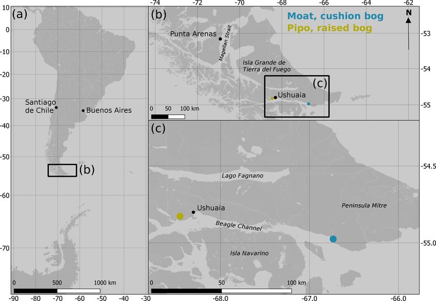
3400                                                          D. Holl et al.: Cushion bogs are strong carbon dioxide net sinks

Figure 1. Location of the two measurement sites Moat and Pipo along the northern coast of the Beagle Channel on Tierra del Fuego,
Argentina. (Map data: © OpenStreetMap contributors 2019. Distributed under a Creative Commons BY-SA License.)

Pleistocene and Holocene periods (e.g., Auer, 1965; Heusser,        of around 40 % (Mark et al., 1995; Lehmann et al., 2016), the
1995; Rabassa et al., 1989, 2000, 2006). More recently, the         most abundant plant species. It occurs in wet lawns and forms
focus of publications in this discipline has shifted towards the    roughly north–south-oriented chains of hummocks perpen-
east (Península Mitre and Isla de los Estados), beyond the ex-      dicular to the drainage direction. Alternating strips of lawns
tent of the last glaciation (Heusser, 1995; Björck et al., 2012;    with pools and hummocks compose most of the peatland’s
Ponce and Fernández, 2014; Ponce et al., 2016). Lately,             surface. The drier hummocks are commonly covered by the
the interest of ecologists in the scarcely studied peatlands        dwarf shrub Empetrum rubrum and the rush Marsiposper-
of Península Mitre has grown (Fritz et al., 2011; Iturraspe,        mum grandiflorum (Lehmann et al., 2016). We found the peat
2012; Grootjans et al., 2014; Münchberger et al., 2019) due         base between 3.8 and 4.3 m below the surface within four
to their pristine character and their spatial dominance in this     peat cores that we drilled at different microtopographical po-
part of Isla Grande.                                                sitions.
                                                                       The literature account of mean annual precipitation for
                                                                    Ushuaia ranges from 530 mm (Iturraspe, 2012), over 545 mm
3     Methods                                                       (Pisano, 1977) to 574 mm (Tuhkanen, 1992). At a central
                                                                    point in the peatland, we measured 515 mm cumulative pre-
3.1     Site descriptions                                           cipitation between 1 March 2016 and 28 February 2017, be-
                                                                    tween 3 % and 11 % below the literature averages. During the
3.1.1    Moss-dominated raised bog, Pipo                            same period, the cumulative evapotranspiration determined
                                                                    with our equipment amounted to 706 mm, making water
Río Pipo mire (hereafter Pipo) is located close to the city
                                                                    stress a considerable issue for plants in 2016. Due to energy
of Ushuaia at 54.83◦ S, 68.45◦ W in Parque Nacional Tierra
                                                                    supply outages, our precipitation records for the remainder of
del Fuego, 60 m above sea level and around 5 km north of
                                                                    2017 and 2018 are incomplete. Precipitation sums measured
the Beagle Channel. The mire is a raised S. magellanicum
                                                                    by the Argentinean Servicio Meteorológico Nacional (SMA)
bog as they are typical for the wind-protected western val-
                                                                    at Ushuaia airport (2016: 334 mm; 2017: 418 mm), which is
leys of Tierra del Fuego (Iturraspe, 2012). It covers an area
                                                                    located around 4 km outside of the city center of Ushuaia
of around 60 ha at the southern end of a glaciogenic valley
                                                                    on a peninsula in the Beagle Channel and close to Centro
bottom. The valley stretches to the southeast and is drained
                                                                    Austral de Investigaciones Científicas (CADIC) in the city
by the river Río Pipo, which marks the northern margin of
                                                                    of Ushuaia (2016: 462 mm; 2017: 520 mm; personal com-
the bog. Along its southern border, a rather narrow lagg zone
                                                                    munication by Gastón Kreps) also suggest that 2016 was a
forms the transition to the adjacent upwards sloping Nothofa-
                                                                    comparably dry year. Deviations between those sums on the
gus pumilio forest. S. magellanicum is, with a surface cover

Biogeosciences, 16, 3397–3423, 2019                                                     www.biogeosciences.net/16/3397/2019/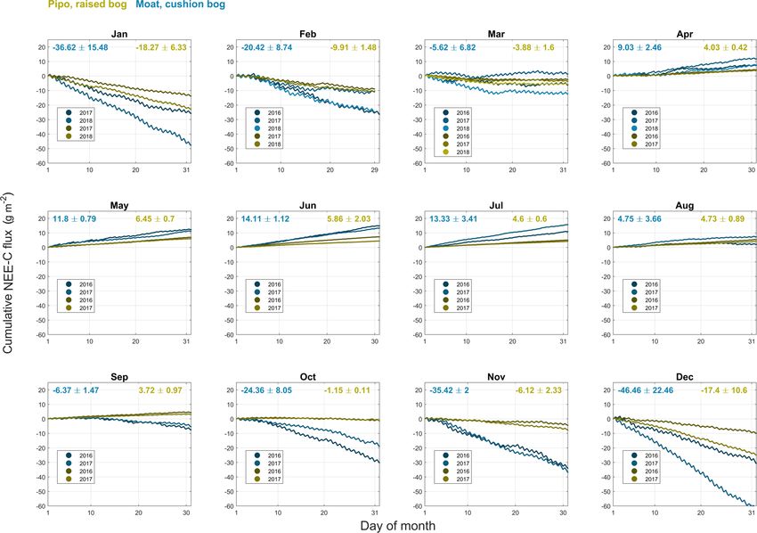
D. Holl et al.: Cushion bogs are strong carbon dioxide net sinks                                                         3401

one hand demonstrate the high variability of local precipita-     2.2 m, thin layers of alternating decomposition grade and de-
tion in the region. On the other hand, sensor bias related to     tritus amount that lack cushion plant remnants occur. From
the windy conditions at the exposed airport site or to the lack   2.2 m to the surface, the substrate consists of highly decom-
of an accurate representation of precipitation as snow could      posed A. pumila peat. At the same site, other studies re-
have contributed to this deviation.                               port similar results. Heusser (1995) found A. pumila resid-
   The mean annual temperature at a long-term meteorolog-         uals until 1.7 m below the surface; Fritz et al. (2011) re-
ical station in Ushuaia is 5.5 ◦ C (Iturraspe, 2012). In 2017,    port Sphagnum peat at depths greater than 3 m. Borromei
we measured an annual mean air temperature of 5.3 ◦ C.            et al. (2014) give a peat depth of 9.96 m that the authors
Mean June air temperatures were 5.8 ◦ C in 2016 and 0.0 ◦ C       date at 9.750 ± 40 years BP. Long-term weather data are
in 2017. Compared to the long-term average June tempera-          not available for Punta Moat. With our setup, we measured
ture of 1.2 ◦ C given by Iturraspe (2012), the winter of 2016     576 mm cumulative rainfall between 1 February and 31 De-
was particularly warm, whereas June of 2017 was closer to         cember 2016 and an annual precipitation of 726 mm in 2017.
the mean. Maximum annual air temperatures occurred on             Mean annual air temperature was 6.27 ◦ C in 2016 (Febru-
26 March 2016 (21.7 ◦ C) and on 6 November 2017 (22.1 ◦ C),       ary to December) and 6.38 ◦ C in 2017. Mean June air tem-
minimum air temperatures on 18 August 2016 (−5.6 ◦ C) and         perature was considerably higher in 2016 (5.41 ◦ C) than in
on 17 June 2017 (−8.1 ◦ C). During both years, wind came al-      2017 (2.07 ◦ C). With a mean February value of 8.90 ◦ C in
most exclusively from west–northwestern directions, hence         2016 and 10.35 ◦ C in 2017 summer air temperatures were
from the valley.                                                  more similar between the years. The highest air tempera-
                                                                  tures were measured on 26 March (22.44 ◦ C) in 2016 and
3.1.2   Vascular plant-dominated cushion bog, Moat                on 6 November (22.48 ◦ C) in 2017, and the coldest air tem-
                                                                  peratures were measured on 2 July (−4.18 ◦ C) in 2016 and
The second site (hereafter Moat) is located close to Bahía        on 17 June (−7.53 ◦ C) in 2017.
Moat at 54.97 ◦ S and 66.73 ◦ W. The bay is formed by the
creek Río Moat that drains towards the south into the Bea-        3.2   Instrumentation
gle Channel at the southwestern edge of Península Mitre.
Our measurements were conducted in a cushion bog approx-          Each eddy covariance (EC) system we used to estimate
imately 1 km off the Beagle Channel’s northern coast, which       turbulent CO2 fluxes consisted of a 3-D sonic anemome-
developed on a series of three glaciofluvial plains elevated      ter (WindMaster Pro, Gill, UK), an infrared gas analyzer
between 33.1 and 40.3 m above mean sea level (Borromei            and a data logger (LI-7200 and LI-7550; LI-COR, USA).
et al., 2014). The bog is limited by Río Moat in the west         Additional atmospheric variables were recorded on a sep-
and a Pleistocene fronto-lateral moraine in the south (Bor-       arate data logger (CR3000; Campbell Scientific, UK). Air
romei et al., 2014). It is sickle-shaped, covers an area of       relative humidity and temperature were measured with an
170 ha and slopes at 0.6◦ slightly towards the southeast. In      HC2-S3 probe (Rotronic, Switzerland), photosynthetically
the north, the mire is bordered by a subantarctic evergreen       active radiation (PAR) with an SKP 215 sensor (Skye Instru-
forest dominated by Nothofagus betuloides and Drimys win-         ments, UK) and precipitation with an ARG100 rain gauge
teri (Heusser, 1995) interlinked with S. magellanicum peat-       (EML, UK). The instrumental setup was identical at both
lands. The cushion bog drains into a channel in the north that    sites. Gas concentrations and three-dimensional wind veloc-
partly runs belowground and receives water from both the          ity raw data were logged at 20 Hz between 31 January 2016
bog and a hill in the north. The outflow channel joins with       and 17 May 2018 in Moat and between 8 February 2016
several other creeks further east before discharging into the     and 17 April 2018 in Pipo. Biomet data were recorded at
Beagle Channel around 4 km southeast of Bahía Moat.               1 Hz within the same time spans. Both LI-7200 analyzers
   More than 70 % (Fritz et al., 2011) of the bog’s surface       were running on factory calibration until 11 November 2017
is covered by the evergreen cushion plants A. pumila and          (Moat) and 9 November 2017 (Pipo), were zero- and span-
D. fascicularis that form dense and firm lawns. They occur        calibrated and restarted on 17 November 2017 (Moat) and
together with Caltha dioneifolia, C. appendiculata, Carex         16 November 2017 (Pipo). Energy to run the equipment
antarctica, Drosera uniflora, Empetrum rubrum, Tetroncium         was generated on-site with a wind turbine (LE-600; Leading
magellanicum and stunted Nothofagus spp. Although the mi-         Edge, UK; peak power 600 W) and two photovoltaic panels
crorelief of this landscape is not very pronounced, a pat-        (OS-172; Leading Edge, UK; peak power 85 W).
tern of cushions and small ponds has developed (Blanco and
de la Balze, 2004). Small areas, often on the somewhat wind-
protected edges of pools, are dominated by S. magellanicum.
In the peat profile, however, remnants of S. magellanicum
make up large parts of the material under areas that cush-
ion plants dominate today. We found Sphagnum peat from
the peat base at 7 until 4.2 m below the surface. From 4.2 to

www.biogeosciences.net/16/3397/2019/                                                    Biogeosciences, 16, 3397–3423, 2019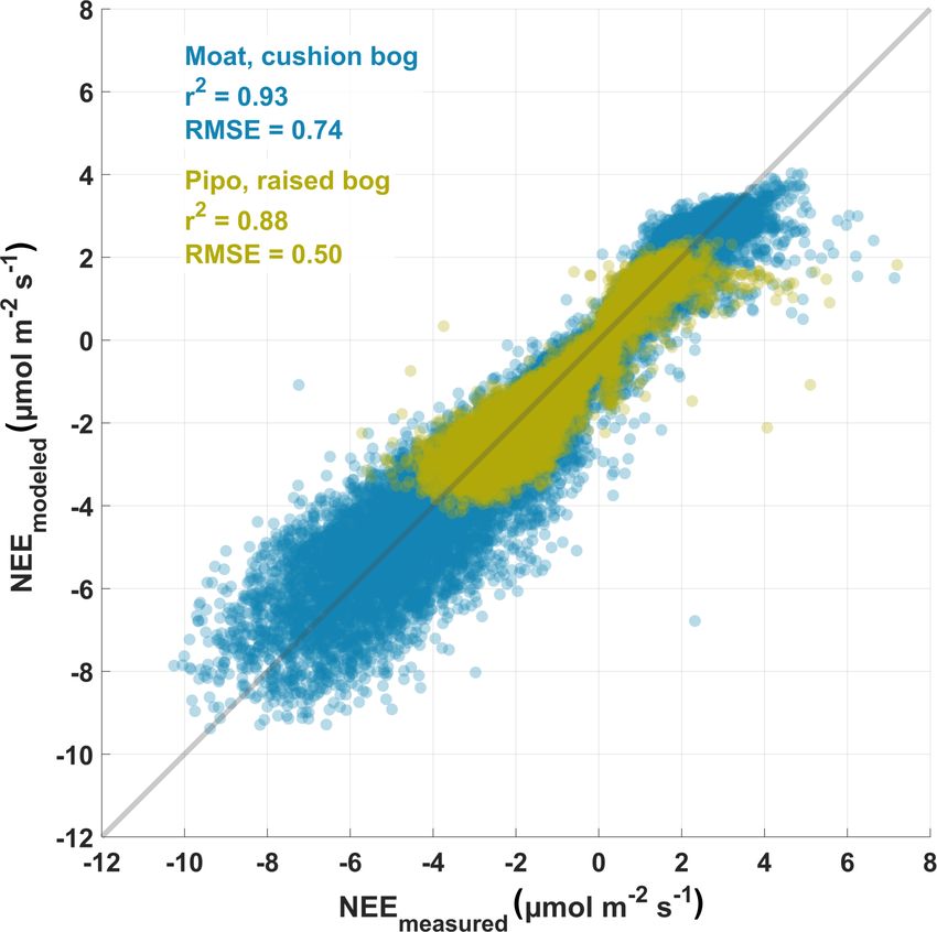
3402                                                         D. Holl et al.: Cushion bogs are strong carbon dioxide net sinks

3.3     Data processing                                            CO2 time lags were not divided in different humidity classes.
                                                                   We addressed time lag statistics later during quality filtering.
3.3.1    Flux calculation and quality filtering                       We corrected for low-frequency loss due to finite aver-
                                                                   aging time and linear detrending as described by Moncrieff
We used the EC technique to determine half-hourly gas and          et al. (2004). In order to obtain a correction factor for each
energy fluxes from the high-frequency raw gas concentra-           flux value, EddyPro estimated true cospectra as proposed by
tion and three-dimensional wind velocity time series. A com-       Kaimal et al. (1972) and reformulated by Moncrieff et al.
prehensive description of the EC approach is given, for ex-        (1997) for each half hour. We set EddyPro to remove high-
ample, by Aubinet et al. (2012). Half-hourly turbulent CO2         frequency noise from the gas concentration spectra before
fluxes were computed using the software EddyPro 6.2.0 (LI-         continuing with the spectral attenuation estimation. In this
COR, USA) and included the following standardized steps;           step, a lower limit of the expected high-frequency noise was
see Holl (2017); Holl et al. (2019).                               user-set. The software then linearly interpolated between this
   We detected and removed raw data spikes according to            lower limit and the highest available frequency (20 Hz) in
Vickers and Mahrt (1997), with a maximum of 1 % accepted           the log–log transformed spectrum and subtracted this func-
spikes and a maximum of three samples as consecutive out-          tion from the spectrum’s high-frequency part. Lower limits
liers. Because we used anemometers that were affected by a         were set to 5 Hz for CO2 and water vapor concentration spec-
firmware bug (published as Technical Key Note KN1509v3             tra. After noise removal, frequency-wise multiplication with
by Gill Instruments), we compensated for the apparent un-          a transfer function yielded an estimate of the filtered signal in
derestimation of the vertical wind speed measurement by in-        the frequency domain. The transfer function was selected by
structing EddyPro to apply the multiplication factor given in      EddyPro according to the detrending method used as given
the mentioned publication. Moreover, due to the use of Gill        by Moncrieff et al. (2004). After integrating over the averag-
anemometers, we applied an angle of attack correction, i.e., a     ing period, a low-cut spectral correction factor for each raw
compensation for flow distortion induced by the anemome-           flux was calculated.
ter frame (Nakai et al., 2006). Coordinate rotation to align          We accounted for high-frequency loss due to path averag-
the anemometer x axis to the current mean streamlines was          ing, signal attenuation and finite time response of the instru-
calculated as double rotation according to Kaimal and Finni-       ments using the method of Fratini et al. (2012). EddyPro first
gan (1994) and linear detrending as proposed by Gash and           determined the cut-off frequency (fc ) and natural frequency
Culf (1996). With simultaneously available water vapor con-        (fn ) by fitting the amplitude response of a first-order low-
centration, cell temperature and cell pressure measurements        pass filter (HIIR (fn /fc )) to power spectrum ensembles of the
from the LI-7200 gas analyzer, CO2 concentrations could            respective scalar time series. For water vapor, fc was esti-
be converted directly into mixing ratios, i.e., concentrations     mated for nine relative humidity classes. Correction factors
referring to dry air of constant temperature (Ibrom et al.,        F 1 were calculated with two methods depending on sensible
2007b; Burba et al., 2012), making corrections for air den-        and latent heat fluxes being above (high fluxes) or below (low
sity fluctuations unnecessary.                                     fluxes) the thresholds of 10 and 5 W m−2 respectively (Fratini
   To determine time lags between the water vapor concen-          et al., 2012). For high fluxes, EddyPro calculated the correc-
tration measurements and the vertical wind speed time se-          tion factors as proposed by Hollinger et al. (1999). F 1 esti-
ries, we used the automatic time lag optimization option in        mation included the degradation of the unattenuated sensible
EddyPro. For this procedure, prior to processing the com-          heat flux cospectrum by multiplying it with HIIR (fn /fc ) for
plete data set, time lags were determined for subperiods of        the previously determined fc . For low fluxes, the obtained
raw data with varying instrumental setup by covariance max-        F 1 fc data set was fitted to the model given by Ibrom et al.
imization (Fan et al., 1990). A searching window around the        (2007a) for stable and unstable conditions. We performed
median of the found time lags (nominal time lag, Tnom ) is         cut-off frequency and function parameter estimation on en-
defined by Tnom ± 3.5 × MAD, where MAD is the median               sembles of (co)spectra separately for two subperiods that
absolute deviation of the found time lags. When processing         we divided at the calibration date (see Instrumentation sec-
the complete data set, EddyPro performed a covariance max-         tion). Before using them for ensemble spectra estimations,
imization of vertical wind speed and the scalar of interest for    the (co)spectra were quality filtered using the scheme of
each half hour and then checked whether the found time lag         Vickers and Mahrt (1997) and by omitting the half hours that
fell within the searching window defined before. If not, Tnom      were assigned quality class 2 according to Mauder and Fo-
was used as time lag. Water vapor concentration time series        ken (2004). We corrected for spectral losses due to crosswind
were binned in 10 relative humidity classes. The procedure         and vertical separation between the LI-7200 tube intake and
was applied to each class, resulting in 10 different nominal       the anemometer in EddyPro following Horst and Lenschow
time lags. Time lags between the CO2 concentration and ver-        (2009). Additionally, we set EddyPro to calculate random
tical wind speed time series were estimated by covariance          flux uncertainty estimates (Finkelstein and Sims, 2001) and
maximization. We calculated time lag statistics and a nom-         three quality flags as proposed by Mauder and Foken (2004),
inal time lag using the above described option in EddyPro.         which represent flux quality in values from 0 to 2, with 0

Biogeosciences, 16, 3397–3423, 2019                                                     www.biogeosciences.net/16/3397/2019/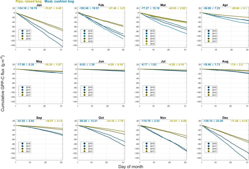
D. Holl et al.: Cushion bogs are strong carbon dioxide net sinks                                                              3403

denoting the highest quality class. This quality evaluation is   method; the cost function that is minimized during optimiza-
based on tests for stationarity and developed turbulence, and    tion is, however, not the sum of squared but of absolute
it thereby indicates whether general EC assumptions about        residuals, reducing the effect of outliers. We used air tem-
atmospheric conditions were met during a flux calculation        perature T (◦ C) and photosynthetically active radiation PAR
period.                                                          (µmol m−2 s−1 ) as independent variables and the quality-
   We performed the following sequence of quality-filtering      filtered CO2 fluxes of Mauder and Foken (2004) classes 0 and
steps on the CO2 fluxes: we evaluated sensor diagnostics by      1 as dependent variable NEE. We set the reference tempera-
using the relative signal strength indication (RSSI) logged      ture Tref , at which TER(Tref ) = Rbase , to 15 ◦ C and γ to 10 ◦ C
from the gas analyzer. Fluxes associated with RSSI values        following Runkle et al. (2013) and Mahecha et al. (2010). We
below 65 were discarded. Furthermore, we excluded fluxes         divided the measured time series in 1, 2 and 5 d intervals and
when a half-hourly time lag, determined with covariance          estimated a set of four parameters for each time window. We
maximization, fell outside the time window around Tnom that      used bounds (Pmax : [0 30]; α: [0 0.05]; Rbase : [0 5]; Q10 : [1
was defined by running the automatic time lag optimization       3]) and start points (Pmax : 5; α: 0.02; Rbase : 1.5; Q10 : 1.4) to
routine in EddyPro (see above). Tnom , as well as the window     constrain parameter optimization. Parameter uncertainty was
size, was determined for subperiods of different analyzer cal-   estimated using their 95 % confidence bounds.
ibration states. To remove remaining outliers, we defined a          In addition to the estimation of NEE fluxes at times when
range of accepted fluxes by using the 0.1st and 99.9th per-      filtered observed fluxes were not available, the bulk modeling
centile of the Mauder and Foken (2004) quality class 0 and 1     approach allows for a decomposition of the net CO2 flux in
fluxes as thresholds.                                            contributions related to photosynthesis and respiration. Be-
                                                                 fore using the bulk model parameter estimates (see Eq. 1)
3.3.2   Net ecosystem exchange partitioning model                for the calculation of modeled NEE, GPP and TER time se-
                                                                 ries, we quality filtered the parameter time series and applied
Unintentional as well as maintenance-related system outages      smoothing functions to them. We rejected all parameters of
and quality filtering of the calculated CO2 fluxes led to gaps   a time window when any of the parameter uncertainty esti-
in the net ecosystem exchange (NEE) data sets. The time          mates were larger than the respective parameter value itself,
series from Moat spans 40 176 half hours with about 12 %         or the algorithm could not ascertain an error estimate indi-
missing records. The Pipo time series is comprised of 38 353     cating a parameter value being stuck at its upper or lower
30 min steps containing 46 % NEE gaps, and this higher per-      bound during iterative optimization. To smooth the parameter
centage of gaps is mainly related to more frequent power         time series, we used a locally weighted regression (Lowess or
outages due to insufficient input through the wind turbine       Loess) method (Cleveland, 1979) in MATLAB. Lowess fit-
and the photovoltaic panels. To be able to calculate annual      ting yields new estimates for the input data that are closer to
C balances from the measured NEE data sets, we gap filled        being members of a continuous function than the input series.
the half-hourly time series with a mechanistic modeling ap-      Lowess smoothing is a stepwise process during which a lin-
proach. We fitted the function given by Runkle et al. (2013)     ear function is fitted to subsets of data around one focal point
to our NEE, air temperature and radiation data. This bulk        for which a new value is estimated as the output of the fitted
model approach is based on the combination of a hyperbolic       function. Line-fitting comprises the assignment of weights to
light saturation function (Thornley, 1998; Zheng et al., 2012)   all used points that increase with their distance from the focal
to represent photosynthesis and an exponential temperature–      point along the x axis (time). The use of second-order poly-
respiration relation (Van’t Hoff, 1898). At times of missing     noms for locally weighted regressions is commonly denoted
NEE observations, the estimated model parameters can be          by the slightly differing abbreviation Loess. We used Loess
used together with temperature and PAR data to estimate          smoothing and quality-filtered results from bulk model esti-
NEE fluxes. Moreover, the net flux can be partitioned in         mates of 2 d windows for all parameter time series except for
its components’ total ecosystem respiration (TER) and gross      Q10 for which we used 5 d window bulk models and first-
primary production (GPP).                                        order polynoms during smoothing. The number of points in-
                            T −Tref
                                                                 cluded in each polynom fit during Lowess or Loess is re-
                                 Pmax × α × PAR                  ferred to as span and was always set to 30 % of all available
NEE(T , PAR) = Rbase × Q10 γ          −
                                 Pmax + α × PAR                  points. As quality filtering of the bulk model parameter esti-
               = TER(T ) + GPP(PAR)                        (1)   mates resulted in unequally spaced parameter time series, we
                                                                 interpolated the smoothed parameter values linearly to 1 d in-
We optimized the four parameters maximum photosynthetic          tervals before driving the bulk models.
rate Pmax , base respiration Rbase (both in µmol m−2 s−1 ),          We assume that seasonal changes in plant-physiological
temperature sensitivity coefficient Q10 and initial quantum      characteristics are more likely to follow a continuous func-
yield α (both dimensionless) using a non-linear least abso-      tion than to exhibit rapid variations. Our method of smooth-
lute residuals method in MATLAB (version 9.5). This algo-        ing the bulk model parameter time series is effective in the re-
rithm is comparable to a traditional non-linear least squares    moval of noise introduced by bulk model fitting that leads to

www.biogeosciences.net/16/3397/2019/                                                     Biogeosciences, 16, 3397–3423, 2019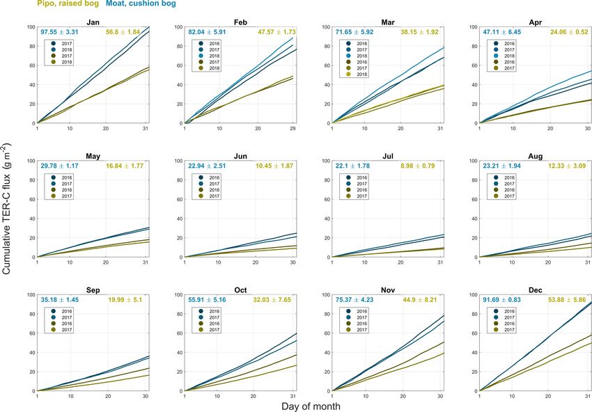
3404 D. Holl et al.: Cushion bogs are strong carbon dioxide net sinks
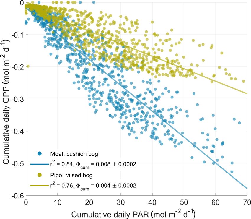
scattering in the parameter time series. Noise characteristics as monthly sums for comparison with monthly respiration
do change with the window size used during bulk model fit- sums. We expressed PARcum as daily sums for comparison
ting, and larger windows lead to less scatter. Window size is with cumulated daily GPP amounts.
then acting as a low-pass filter that potentially smears up pos-
sibly inherent parameter changes on shorter timescales that 3.3.4 Calculation of annual net ecosystem exchange
are, in contrast, still intact after Lowess or Loess smoothing. sums
Shorter-term variations, for example synoptic-scale changes
of environmental conditions, can lead to short-term adaption We proceeded to drive daily versions of Eq. (1), each com-
of plants that should be reflected in bulk model parameter prised of a distinct set of four parameters, with half-hourly,
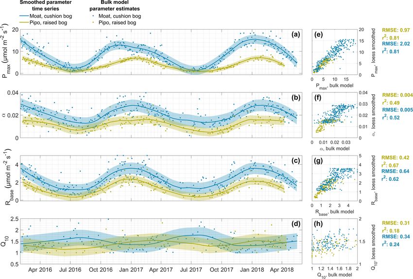
time series. The changes in Moat Pmax curvature in summer gap-filled radiation and temperature data. We calculated un-
of 2016–2017 (see Fig. 2) are an example of the smoothed certainty estimates uGPP , uTER and uNEE for each modeled
parameter series’ abilities to reflect inter-annual variations of GPP, TER and NEE flux based on Gaussian error propaga-
the seasonal parameter course, in this case a prolonged phase tion and representing a 95 % confidence interval. We took the
of unusually cloudy conditions in Moat during early summer partial derivatives of Eq. (1) with respect to the four parame-
in December (see Appendix, Fig. C1). ters as described in the Appendix (Eqs. A1 to A3). We sim-
To estimate a PAR value at which the canopy photosyn- plified the process by neglecting comparably small random
thetic potential was reduced to 1/10 of its initial value α, and errors in temperature and radiation measurements. We used
therefore near saturation, we calculated PARsat as the root mean square error (RMSE) of the smoothed daily
r parameter time series and the quality-filtered bulk model pa-
P2
4 αmax 2 1−zsat rameter assessments as uncertainty estimates for each value
2 − 4Pmax 2
Pmax α
of the smoothed parameter series.
PARsat (Pmax , α) = + , (2)
α 2 The partitioned NEE time series from Moat contains data
using the previously determined Pmax and α time series at from 29 months (838 d), and the Pipo data set includes
1 d intervals and an attenuation factor zsat of 10. To set up records from 27 months (800 d). For the analysis of annu-
Eq. (2), we differentiated Eq. (1) with respect to PAR and set ally accumulated fluxes, we only used months for which gap-
it equal to a by 1/10 attenuated quantum use efficiency. We filled data were available at each half hour of each day. We
solved this equation for PAR to calculate PARsat time series used these 27 (Moat) and 25 (Pipo) complete months to in-
for both sites. Details are given in Appendix D. vestigate inter-annual variability at each site as well as gen-
eral variability between the sites.
3.3.3 Processing of ancillary meteorological variables We constructed an average annual course from spring
(1 September) to winter (31 August) by calculating mean
Before the half-hourly NEE simulations, we filled gaps in monthly sums of NEE, GPP and TER (see Figs. B1, B2 and
the 30 min PAR and air temperature records. We applied a B3). Complete monthly records were mostly available from
mean diurnal variation method similar to the approach of 2 years, and three full monthly records were available for
Falge et al. (2001), which exploits the commonly high auto- March at Pipo as well as for February, March and April at
correlation of these meteorological variables. Missing values Moat. We expressed the range of individual monthly sums
were replaced by averages of available records at the same as standard deviation. In most cases, when n = 2, this means
hour of the day within increasing time windows between 1 that the range is expressed as the absolute difference between
and 7 d around a gap. Window size was increased until at both values divided by the square root of 2. To estimate and
least one record could be found. If more than one record compare average annual courses of the vertical CO2 balances
was available, an average was used to fill the respective gap. between both sites, we cumulated the 12 average monthly
Within the Pipo data set, 7 % of meteorological observations sums. We also added together the standard deviations related
were missing, and 92 % of these values were filled with aver- to each of these sums to indicate the impact of variations be-
ages. The Moat time series contained 1 % gaps, and in 93 % tween years on the annual balances. By adding the monthly
of all cases more than one record was found within the time range estimates and not using the root of the sum of their
window around a gap. Gap filling was mostly (70 %) per- squares, we treated them as potentially systematic rather than
formed using 1 d windows for the Pipo data set and with 1 to random variations of annual NEE, GPP and TER sums.
3 d windows in most cases (57 %) of the Moat time series. To investigate the effect of changing environmental con-
Data analysis included the calculation of the cumulative ditions on the partitioned NEE balances at both sites, we di-
temperature and radiation quantities growing degree days vided the time series into 2 consecutive years that we will
(GDD) in degrees Celsius and cumulative photosyntheti- term Y1 and Y2 hereafter. Because the observations spanned
cally active radiation PARcum in moles per square meter a bit more than 2 years at both locations, we additionally
(mol m−2 ). We defined GDD5 as the sum of all positive dif- checked the effect of choosing different start dates for 12
ferences between daily average temperatures and a reference month intervals that represent various versions of Y1 and
temperature, which we set to 5 ◦ C. GDD5 was calculated Y2. We defined three start dates (Pipo: 1 March and 1 April;
Biogeosciences, 16, 3397–3423, 2019 www.biogeosciences.net/16/3397/2019/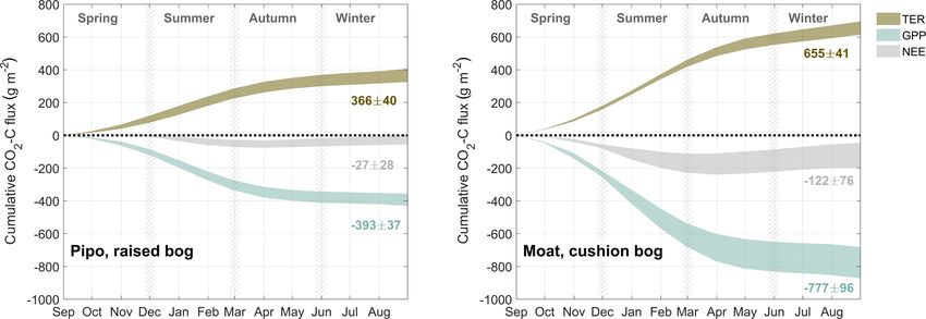
D. Holl et al.: Cushion bogs are strong carbon dioxide net sinks                                                         3405

Moat: 1 February, 1 March and 1 April), yielding two (Pipo)      indicated by the lower level of Pmax , Rbase and α values
and three (Moat), in large parts overlapping versions of Y1      throughout the course of both years in Pipo. Moreover, the
and Y2 per site.                                                 timings of the slope changes within these parameters se-
   Estimated GPP and TER fluxes contain only bulk model          ries demonstrate that cushion plant photosynthetic activity
results, NEE fluxes include measurement data of quality          reaches its maximum earlier in summer compared to the
class 0 and modeled fluxes at times without highest-quality      moss-dominated community, while inter-annual variations
observations. Random uncertainty of the observed fluxes was      also lead to variations of this time lag. While Pmax max-
estimated using the method of Finkelstein and Sims (2001)        ima were reached about 6 weeks earlier in Moat (28 Novem-
(see Sect. 3.3.1), and modeled fluxes were assigned the pre-     ber 2016) than in Pipo (13 January 2017) in summer of Y1,
viously determined uGPP , uTER and uNEE values as uncer-         Moat Pmax maxima (8 January 2018) were about 3 weeks
tainty estimates. The uncertainty of the annual balances was     ahead of Pipo (28 January 2018) in summer of Y2. Rbase
calculated by taking the square root of the sum of squared       maxima time lags were less pronounced and amounted to
individual 30 min flux uncertainties.                            about 10 d in Y1. In contrast to the timing of Pmax maxima,
                                                                 Rbase maxima were reached earlier at Pipo. In summer of
                                                                 Y2, Moat and Pipo base respiration developed virtually con-
4     Results and discussion                                     currently. While Q10 Lowess estimates are the least certain
                                                                 compared to the three other parameters, smoothing reveals a
4.1    Quality filtering
                                                                 contrasting, mirrored behavior of the sensitivity of respira-
Quality filtering of the measured data resulted in 5 % and       tion to temperature changes between both sites. While Q10
13 % omitted records from Moat and Pipo respectively. Most       maxima occur in winter and minima in summer throughout
fluxes (1786 and 3105) were filtered out due to the time lag     all years in Moat, Pipo Q10 reaches its maxima in summer
detection quality filter. Of the remaining 36 363 and 22 037     and its minima in winter. However, the Q10 value ranges we
points, 81 % and 71 % were of Mauder and Foken (2004)            found are small, which is in line with results from Mahecha
quality class 0, and 97 % and 95 % were of combined quality      et al. (2010), who reported that ecosystem level temperature
classes 0 and 1.                                                 sensitivity of TER is with 1.4 ± 0.1 rather stable across dif-
   Quality filtering of the bulk model parameter time series     ferent global ecosystems.
resulted in 290 Pmax , α and Rbase values from 2 d window fits
for Moat and 155 for Pipo. Related to the total number of 2 d    4.3   Flux gap filling and partitioning
windows spanned by the time series, data coverage amounts
to 69 % and 34 % for Moat and Pipo respectively. In case of      After Lowess or Loess smoothing, we interpolated the bulk
the 5 d intervals used for the estimation of Q10 time series,    model parameter time series to equally spaced 1 d intervals
85 and 140 values met the quality criteria equaling 84 % and     and proceeded to drive those daily models with half-hourly
53 % of all 5 d intervals within the NEE time series.            meteorological data. We used the resulting NEE time se-
                                                                 ries to gap fill the observed data sets enabling us to esti-
4.2    Bulk model parameter time series                          mate annual vertical partitioned CO2 balances of both bogs.
                                                                 The gap-filled NEE data sets consist of quality class 0 mea-
We applied Lowess or Loess smoothing to the parame-              sured fluxes and 26 % (Moat) and 59 % (Pipo) modeled
ter time series and thereby generated new sets of bulk           fluxes. Agreement between eddy covariance net CO2 fluxes
model parameters. Smoothed and original bulk model pa-           and modeled fluxes is high while RMSEs are low (Moat:
rameters are compared in Fig. 2. The results generally           0.74 µmol m−2 s−1 ; Pipo: 0.50 µmol m−2 s−1 ) as illustrated
show good agreement with the highest coefficient of de-          in Fig. 3. The models can not explain a relatively small
termination (r 2 ) of 0.8 for Pmax at both sites, r 2 val-       amount of measured high positive fluxes at both sites, which
ues between 0.5 and 0.7 for α and Rbase , and lowest r 2         could possibly be related to the rapid release of bubbles from
values of 0.2 in case of Q10 . Loess/Lowess model un-            ponds (ebullition; e.g., Glaser et al., 2004). Deviations be-
certainty, estimated as RMSE, ranges between 22 % and            tween model and measurement data increase with increas-
29 % of the respective mean parameter value across both          ing absolute fluxes and are smaller close to zero. Bias errors
sites and parameter sets. Bias errors, expressed as sum          (BEs), expressed as sum of differences between measured
of differences between bulk model and smoothed data              and modeled data points divided by the number of samples,
points divided by the number of samples, are negative and        are positive but low for both sites (Moat: 0.05 µmol m−2 s−1 ;
small for both sites (Pipo: Pmax : −0.03 µmol m−2 s−1 , α:       Pipo: 0.04 µmol m−2 s−1 ). The much smaller value range of
−0.00008, Rbase : −0.01 µmol m−2 s−1 and Q10 : −0.002;           CO2 fluxes from Pipo compared to Moat is also apparent in
Moat: Pmax : −0.03 µmol m−2 s−1 , α: −0.00006; Rbase :           Fig.3. Furthermore, we determined correlation coefficients
−0.007 µmol m−2 s−1 and Q10 = −0.003).                           between the modeled TER time series and nighttime (PAR <
   General differences in ecosystem characteristics between      10 µmol m−2 s−1 ) EC NEE fluxes and found that also this
the cushion plant-dominated and moss-dominated site are          partitioned flux was well explained by our model (Moat:

www.biogeosciences.net/16/3397/2019/                                                   Biogeosciences, 16, 3397–3423, 2019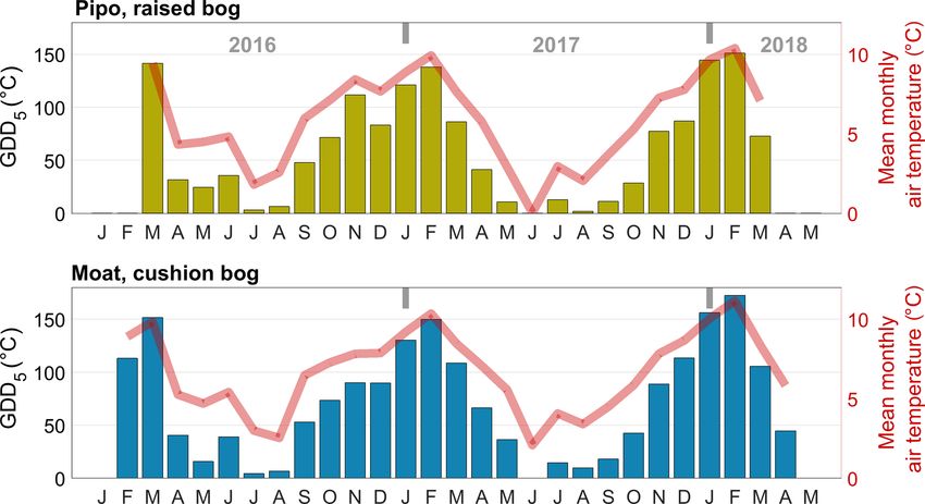
3406                                                            D. Holl et al.: Cushion bogs are strong carbon dioxide net sinks

Figure 2. Time series of the parameters maximum photosynthesis Pmax (a), initial quantum yield α (b), base respiration Rbase (c) and
temperature sensitivity Q10 (d) that we estimated with 2 d, and in case of Q10 with 5 d, window NEE bulk models (dots) and smoothed
with a locally weighted regression (Lowess or Loess) method (lines). Areas around lines indicate the uncertainty of smoothed parameter
values. Correlations between original bulk model estimates and smoothed values are shown in panels (e) to (h) including the coefficients of
determination (r 2 ) and root mean square error (RMSE).

r 2 = 0.8, n = 14 887, RMSE = 0.43 µmol m−2 s−1 , BE =                  June temperatures at Pipo were 4.6 ◦ C above the long-term
−0.003 µmol m−2 s−1 ; Pipo: r 2 = 0.6, n = 6081, RMSE =                 average (Iturraspe, 2012). Only at Pipo, early summer of the
0.40 µmol m−2 s−1 , BE = −0.08 µmol m−2 s−1 ).                          next vegetation period (November 2016, still in Y1) was once
                                                                        again warmer than the average. With respect to cumulatively
4.4    Inter-annual flux and driver variability                         available heat, these temperature variations led to a decrease
                                                                        in GDD5 of around 16 % at Pipo in Y2, whereas GDD5 rose
To investigate the inter-annual variability of GPP and TER,             by less than 1 % at Moat, which is located closer to the coast.
we cumulated the modeled half-hourly time series annu-                  The raised bog’s ecosystem respiration was modulated more
ally for different versions of Y1 and Y2 as described above             strongly by the warmer conditions in Y1 than by photosyn-
(Sect. 3.3.4). To estimate changes in cumulative NEE fluxes,            thesis that dropped only by around 2 % in Y2. However, pho-
we used gap-filled EC fluxes and summed them up over the                tosynthesis was also seemingly promoted by the larger avail-
same time periods. We calculated mean annual balances from              ability of heat in Y1, as despite the cumulative radiation in-
the different versions of Y1 and Y2 (see Table 1). To put the           crease by about 4 % in Y2 at Pipo, cumulative |GPP|1 still
balances into context with shifts in meteorological drivers             dropped. The annual PAR sum increased more strongly, by
of photosynthesis and respiration, we calculated the monthly            about 10 %, at the cushion bog site where we estimated a 5 %
cumulated temperature and radiation measures GDD5 and                   rise in cumulative |GPP|. As mentioned before, close to the
PARcum (see Figs. C1 and C2 in the Appendix).
   In 2016, growing season temperatures peaked in March,                   1 Following micrometeorological conventions, we use GPP with
about 1 month later than in the two other observed sum-                 a negative sign as the associated CO2 flux is directed from the at-
mers. This vegetation period shift continued with an unusu-             mosphere towards the surface. We use absolute values to be able to
ally warm late summer and autumn and culminated in an                   describe a decrease or increase in the process photosynthesis with a
extremely warm winter month of June at both sites. Mean                 decrease or increase in |GPP|.

Biogeosciences, 16, 3397–3423, 2019                                                           www.biogeosciences.net/16/3397/2019/
D. Holl et al.: Cushion bogs are strong carbon dioxide net sinks 3407
month used for summing has a larger impact on annual C up-
take at Moat than at Pipo. While NEE-C uptake changes from
Y1 to Y2 range from a decrease of 2 g m−2 to an increase of
47 g m−2 at Moat, the choice of different start months leads
to less variability (NEE-C uptake increases from Y1 to Y2
between 23 and 27 g m−2 ) at Pipo.
Apart from differences in inter-annual variations of an-
nual NEE sums between the sites, distinctions also arise with
respect to the variability of monthly sums from different
years. Variations within monthly NEE component sums (see
Figs. B1, B2 and B3 in the Appendix) are most pronounced at
Moat with respect to GPP and at Pipo with respect to TER. In
December, the |NEE|-C differences between 2016 and 2017
are large at both sites (Moat: 32 g m−2 ; Pipo: 15 g m−2 ). Al-
though GDD5 was considerably larger only at Moat in De-
cember 2017, the relative rise of TER from December 2016
to December 2017 was small (1 g m−2 ). At Pipo, where
GDD5 increase was smaller from December 2016 to Decem-
ber 2017, TER-C loss dropped by 8 g m−2 . November 2016
was particularly warm at Pipo, and the effects might have car-
ried into December. The monthly PAR sum increased from
Figure 3. Scatter diagram of modeled half-hourly measured eddy
December 2016 to December 2017 at both sites and led to an
covariance net ecosystem exchange (NEE) fluxes and modeled NEE
fluxes, which were derived using Eq. (1). Coefficient of determina-
increase in GPP-C uptake of 33 g m−2 at Moat and of 7 g m−2
tion (r 2 ) and root mean square error (RMSE) are given for both at Pipo. Monthly NEE-C balances of Pipo appear to deviate
investigation sites (Pipo, n = 15 903; Moat, n = 29 648). more intensively from an average annual course when de-
viations from a mean annual temperature course occur con-
currently. At Moat, the GPP response to deviations from the
mean in the available amount of PAR has an overriding ef-
coast, the summer of Y1 apparently was considerably more fect on variations of monthly NEE-C balances. While TER is
cloudy than the subsequent season (see Fig. C1 in the Ap- generally at a higher level at Moat compared to Pipo, inter-
pendix). From Y1 to Y2 , net CO2 uptake increased on aver- annual temperature variations within months have a less pro-
age by 35 % in Moat and more than tripled in Pipo. In terms nounced relative impact on the mean seasonal course of TER.
of absolute CO2 uptake increase, the rise at Moat was, how- On average, net CO2 uptake increased substantially at both
ever, larger than at Pipo, denoting the fact that CO2 fluxes are sites from Y1 to Y2. However, this similar net change re-
on a lower level at Pipo in general. Y1 was an extreme year, sulted from contrasting magnitudes and directions of changes
especially at Pipo, where prolonged warm temperatures (see of GPP and TER at both sites. Table 2 gives a simplified,
Fig. C1 in the Appendix) and reduced precipitation likely led coarsely abstracted overview of the differences in averaged
to dry topsoil conditions that promoted heterotrophic respi- cumulated flux and driver quantities between Y1 and Y2 and
ration diminishing the ecosystem’s CO2 sink function in this from site to site; detailed results are given in Table 1 and
year. Figs. C1 and C2 in the Appendix. From Y1 to Y2, the mag-
The values of all cumulative NEE fluxes and their compo- nitude of GPP and TER increased at Moat while |GPP| and
nents that were used to calculate averages from different ver- TER decreased at Pipo. The reduction of cumulative respira-
sions of Y1 and Y2, distinguished by various start months, tion at Pipo was, however, larger than the drop in the |GPP|
are given in Table 1. The largest difference in annual NEE sum, leading to an increase in annual net CO2 uptake. At
sums between Y1 and Y2 arises in case of the Moat data set Moat, the rise in |NEE| traces back to an increase in |GPP|
when February and March 2016 are excluded from Y1, and that was larger than the simultaneous ascent of respiration.
accordingly the same months of 2018 are included in Y2.
Late summer 2015–2016 was characterized by cool temper- 4.5 Average annual fluxes
atures and less available radiation than summer 2017–2018
when we measured the highest radiation sums and modeled As a way to ascertain general site differences in CO2 flux pat-
highest cumulative |GPP| within the observed time series. terns, we used all available full months to construct average
Excluding an extreme event in the first year and at the same annual courses of NEE and its components GPP and TER.
time including a period with an opposite effect on the net We calculated monthly sums of all fluxes (see Figs. B1, B2
CO2 flux in the second year maximizes the differences be- and B3) and averaged these sums across all available records
tween both years at both sites. The choice of a particular start of each month. We summed up these monthly averages over
www.biogeosciences.net/16/3397/2019/ Biogeosciences, 16, 3397–3423, 2019You can also read