Modelling clouds for weather, climate and beyond - Ian Boutle + many collaborators - University of ...
←
→
Page content transcription
If your browser does not render page correctly, please read the page content below
Modelling clouds for
weather, climate and
beyond...
Ian Boutle
+ many collaborators...

www.metoffice.gov.uk      © Crown Copyright 2018 Met Office

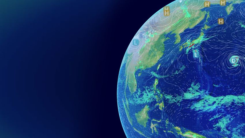
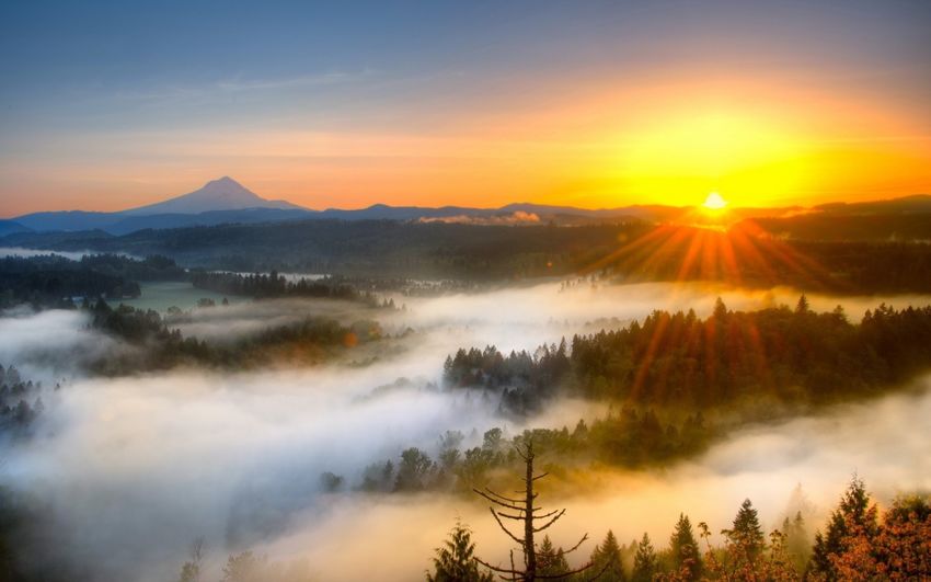
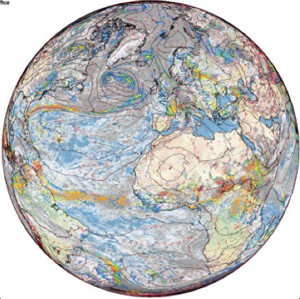
The real world is complex...
• Computer
  models used for
  weather
  forecasts and
  climate
  simulations need
  to represent all of
  this complexity.

• BUT, they need
  to do so in a very
  efficient
  manner...
Du               Ñp
                                                        = -2Ω × u -     + g + Su
                                                   Dt                r
                                                               ¶r
The forecast problem                                              + Ñ.( r u) = 0
                                                               ¶t      Dq
• Core of the model solves the Navier-Stokes equations                     = Sq
• Must discretise these onto a finite-difference grid to solve         Dt
                                                                      p = r RT
• Weather forecasts take 30-60 minutes (of computer time)
   • Anything shorter, you may as well do things better
   • Anything longer ceases to be a forecast
• Current global forecast model runs on 4752 processors
   • New supercomputer (Cray XC40) installed in 2016
• So to fit a 7-day forecast into those resources, we can afford 2560 x 1920
  x 70 grid points – approx 10km horizontal resolution!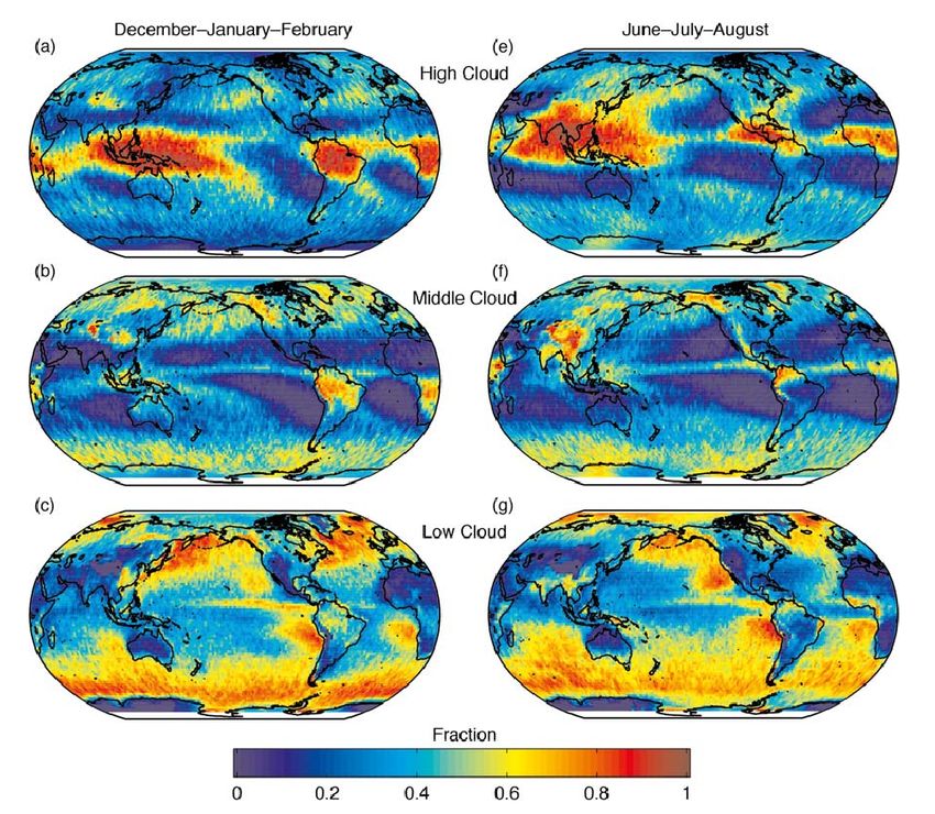
Du             Ñp
                                                                     = -2Ω × u -    + g + Su
                                                                  Dt             r
The parametrization problem                                                        Dq
                                                                                       = Sq
                                                                                   Dt
• Many processes exist on a scale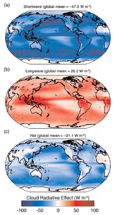
Contents
1. Very high-resolution modelling for aviation at Heathrow airport
2. Cloud parametrization improvements for the latest climate model
3. Beyond Earth – adapting the model for exoplanet atmospheres

www.metoffice.gov.uk                                                 © Crown Copyright 2018, Met Office
1. Very high-resolution modelling for aviation at
Heathrow airport
Heathrow and fog
• Heathrow is one of the busiest airports in the world – runs at ~99%
  capacity
• When visibility is low, space between aircraft must be increased -> lower
  capacity -> cancelled flights
• 75% of delays are weather related, half of this is due to low visibility
• Very expensive + lots of grumpy passengers
• With accurate forecasts, can plan ahead to mitigate the effects
• How can we improve our forecast accuracy?
Model hierarchy
GM -               UKV – 1.5km   • Don’t just run 10km
10km                               global model
                                 • Region of interest
                                   is UK, so nest a
                                   1.5km model inside
                                   this
                                 • HUGE benefit in
                                   detail and accuracy
                                 • What if we added
                                   another level?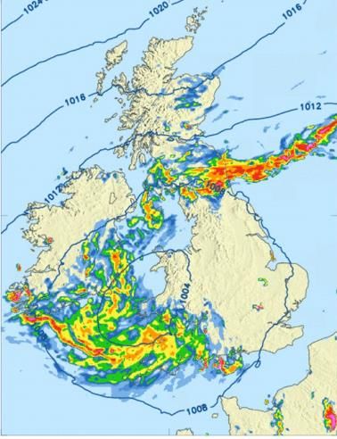
• Enhanced detail in terrain features,
                                land-surface characteristics
                              • Better resolution of atmosphere
The London Model              • Less reliance on parametrizations
    333m                             1.5km

           Heathrow Airport     London City Airport

                                                      Boutle et al. (2016, QJRMS)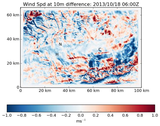
An example from last
winter:
• The enhanced resolution
                           genuinely alters the evolution of
                           the fog
Not just an HD picture
                         • Why?

                                           Boutle et al. (2016, QJRMS)
• Use the lower resolution
orography field from the UKV in
the LM, gives big change in fog
Smoothed terrain evolution
Boutle et al. (2016, QJRMS)A turbulence feedback
• Rougher terrain strongly affects the
near surface wind field
• This extra variability in the wind-
shear affects the structure of the
atmosphere:
• More turbulent
• Extra turbulence mixes warmer air down
from aloft
• Warmer air prevents fog formation
LM difference – (rough – smooth) • A genuine benefit of higher
resolution, but could we
parametrize it at lower resolution?
Boutle et al. (2016, QJRMS)2. Cloud parametrization improvements for the latest climate model
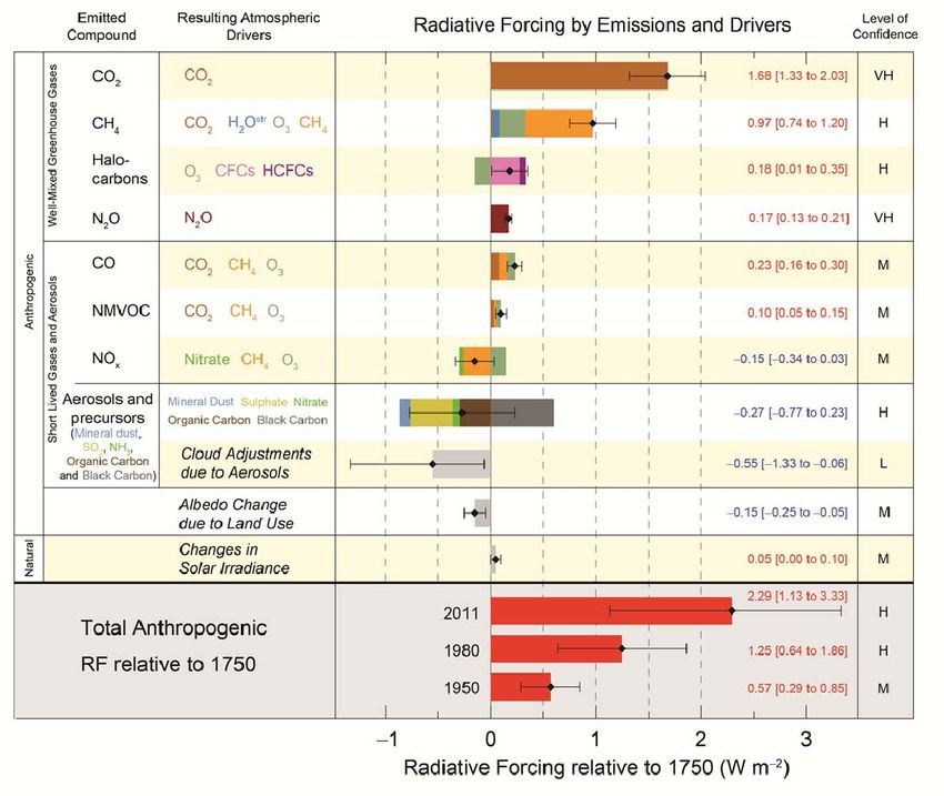
Clouds and climate
                      • Clouds represent the single biggest
                        uncertainty in climate models
                      • How they respond to a warming
                        climate could EITHER significantly
                        reduce the amount of warming OR
                        significantly increase it!
                      • Hence a strong requirement to
                        improve their modelling

IPCC AR5
Existence and effect in the climate system
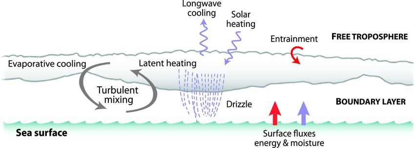
Low clouds are the
most prevalent cloud
type on the planet
They provide a
cooling to the climate
system
Whether there are
more (wetter) or less
(warmer) of them could
create a negative or
positive feedback• Combination of many different
physical processes
Why is modelling low • Most of which are parametrized
• Fundamental physics of many is
clouds so difficult? poorly understood
Wood (2012, MWR)“Dreary” state of precipitation in climate
models
• CloudSat sees the cloud and precipitation falling below it
• Higher reflectivity -> bigger drops
Obs Model
Continuous Two distinct
transition modes –
from cloud one for
to rain cloud, one
for rain
• Not unique to our model! Bodas-Salcedo et al, (2008, JGR)Microphysical
modelling
• Equations for droplet growth are well known
and understood – easy to solve
• Each grid-box contains a spectrum of particles
of different sizes
• Could model each different sized particle
explicitly – bin scheme (too expensive ~30+
prognostic variables)
Abel & Boutle (2012, QJRMS)Rain drop size distribution
• Hence have to assume a size distribution of
particles and integrate over it – bulk scheme (2
prognostic variables, cloud water & rain water)
• Assume the number of rain-drops (N) is related
to their diameter (D) by:
N ( D) = N 0 exp(-lD)
• Most models use Marshall & Palmer (1948):
N 0 = 8 ´10 6
• Doesn’t appear to match reality very well…
Abel & Boutle (2012, QJRMS)Relationship between N0 and rain-rate
• Many in-situ aircraft observations +
surface radar/lidar/distrometer
observations
• Suggests a relationship between N0
and λ:
N 0 = 0.22l 2.2
• λ is a physical quantity, related to the
total mass of rain
N 0 = 8 ´106
Abel & Boutle (2012, QJRMS)How precipitation physics depends on this
• Evaporation of rain-drops • Fall-speed of rain-drops
New-method
greatly
improves this
OLD NEW
Old-method over- New-method
Old-method under-estimated the estimated the fall- greatly
evaporation rate speed improves this
Abel & Boutle (2012, QJRMS)Rain creation processes
• Conversion of cloud to rain treated by a simple
power-law:
OLD
¶ (qrain)
= C (qcl ) A ( N d ) B
¶t
• qx=mass of cloud/rain, Nd=number of cloud
droplets NEW
• A, B & C are empirically determined constants
• Old scheme (TC) over estimated rain-creation
compared to observations – replace with new
scheme (KK)
Wood (2005, JAS)Do we understand this?
Obs Model
Continuous Two distinct
transition modes –
from cloud one for
to rain cloud, one
for rain
• Model over-estimates rain creation, over-estimates rain fall-speed, under-
estimates rain evaporation...
• Un-surprising that there is excessive rain and two distinct modes.Zoom in on the low cloud
Obs Old Model
Boutle & Abel (2012, ACP)• Slower rain-creation lowers the
peak reflectivity produced as
rain is forming
Zoom in on the low cloud
Obs New Model
• Slower fall-speed and more evaporation stops fast falling to the
surface and gives reduction in reflectivity below cloud
Boutle & Abel (2012, ACP)Old
But...
There’s a
problem
Low resolution – Intermediate High resolution
climate model
• Old climate model actually gave the correct mean surface rain-rate
• Cloud processes are highly nonlinear, so increasing model resolution
increases the surface rain-rate (to excessive amounts)
Boutle et al. (2014, MWR)Old
But...
There’s a
problem
Low resolution – Intermediate High resolution
climate model
• What I’ve just showed you was fixing the high-
resolution version
• Applying the same thing at low resolution would
significantly under-estimate the rain-rate!
New
Boutle et al. (2014, MWR)Back to rain creation
• Already showed earlier that rain creation is parametrized as:
¶ (qrain)
= C (qcl ) A ( N d ) B OR For simplicity
¶t
• In a climate model, we want the grid-box averaged process rate (M), but
only have the grid-box averaged q
• Hence for b≠1:
M = aq ¹ aq b b
• This introduces a systematic bias into the modelAnalytically correcting the process rates • Suppose we have some information about the sub-grid distribution of q, e.g. that it can be represented by a log-normal distribution: • Then we can integrate over the PDF to obtain: • We can improve our estimate of M by just knowing f and the PDF shape
Parameterizing the variability (f)                 • Variability
                                                     increases
                                                     with scale
                                                   • Biggest
                                                     change at
                                                     smallest
                                                     scales
                                                   • Variability
                                                     also
                                                     effected by
                                                     cloud size
                                                     (smaller ->
                                                     more
                                                     variable)

                                     Boutle et al. (2014, QJRMS)
Process rate bias
• At a given scale (here ~50km),
compute the exact process rate
from high-resolution data, and
the process rate based on mean
inputs
• Exact rate is under-estimated by
a factor of ~4
• Correction is almost exact using
PDF method and observed f
• And very good using
parametrized f
Boutle et al. (2014, QJRMS)Old
Problem
solved!
• Now the rain
rate is Low resolution – Intermediate High resolution
approximately climate model
constant,
regardless of
resolution!
New
Boutle et al. (2014, MWR)New climate model
New
• Include these changes in the new climate model
Model
• Transition of cloud to rain is significantly improved
• Greater confidence that model is doing the right
thing for the right reason
Obs
Obs Old
Model
Walters et al. (2017, GMD)3. Beyond Earth – adapting the model for exoplanet atmospheres
Diversity of the universe
• In the early 1990’s, the first planet orbiting a star other than the sun was
  found
• Since then, 3584 such planets have been found:
   •   1418 Neptune-like
   •   1205 Gas giant (Jupiter-like)
   •   883 Terrestrial (Earth-like)
   •   53 Super-earth (somewhere between Earth and Neptune)
• Modelling provides a method of interpreting the (limited) observations,
  understanding the planetary universe, and hunting for life...
Wind

  Hot Jupiters
  • Best observed – large gas giants orbiting very
    close to parent star – tidally locked – same side
    always facing the star
  • Some observations of temperature (~1000 K)
    and wind-speed (~5000 m/s)
  • Change the stellar-spectra and planetary
    parameters (orbit, mass, radius, ...) and the                     Temp
    model can produce a credible simulation of this
    environment!
  • Raises all sorts of further questions about
    structure of the atmosphere - at this
    temperature metal species (e.g. TiO2) will
    condense                                            Night   Day

Lines et al. (2018, A&A)
Cloud
Cloudy exoplanets
• Couple model to metallic cloud
formation code developed at St
Andrews University Night Day
• Produce simulated observations from
model and compare to actual
observations
• Cloudy model is better fit than clear
sky, but differences suggest the
physics is still incomplete
• Role of chemistry?
Lines et al. (2018, A&A)Terrestrial planets
• The holy-grail, but observations currently
limited to “it’s this big, in this orbit” – nothing Surface Temp
about structure or composition of
atmosphere
• Doesn’t stop us speculating!
• E.g. Proxima Centuari B - ~Earth mass
planet orbiting our nearest star
• Given an Earth-like atmosphere (N2, CO2,
H2O), modelling suggests planet would
Cloud
have temperate climate and liquid water
Boutle et al. (2017, A&A)How might we know?
• Plenty of interesting science that can be done
studying the climate of such a planet
• Key question though is how would we ever
know?
Oxygen
• Again, can produce simulated observables
(the kind that could be possible with future
telescopes).
• Small changes to the atmosphere can show
up the signals of important gases, e.g. Ozone
and Oxygen
Ozone
Boutle et al. (2017, A&A)Conclusions The same (very large) code can be used for highly detailed simulations of small parts of this planet, to planetary scale simulations of gas-giants many light years away Efficiency is a key driver – we’re always doing the best we can with the computer time we have available www.metoffice.gov.uk © Crown Copyright 2018, Met Office
You can also read


