Method to Adjust ITE Vehicle Trip-Generation Estimates in Smart-Growth Areas
←
→
Page content transcription
If your browser does not render page correctly, please read the page content below
Method to Adjust ITE Vehicle Trip-Generation
     Estimates in Smart-Growth Areas
         Robert J. Schneider, Kevan Shafizadeh, & Susan L. Handy
     University of Wisconsin-Milwaukee, CSU Sacramento, & UC Davis
       TRB Innovations in Travel Modeling Conference—April 2014

                                                                     1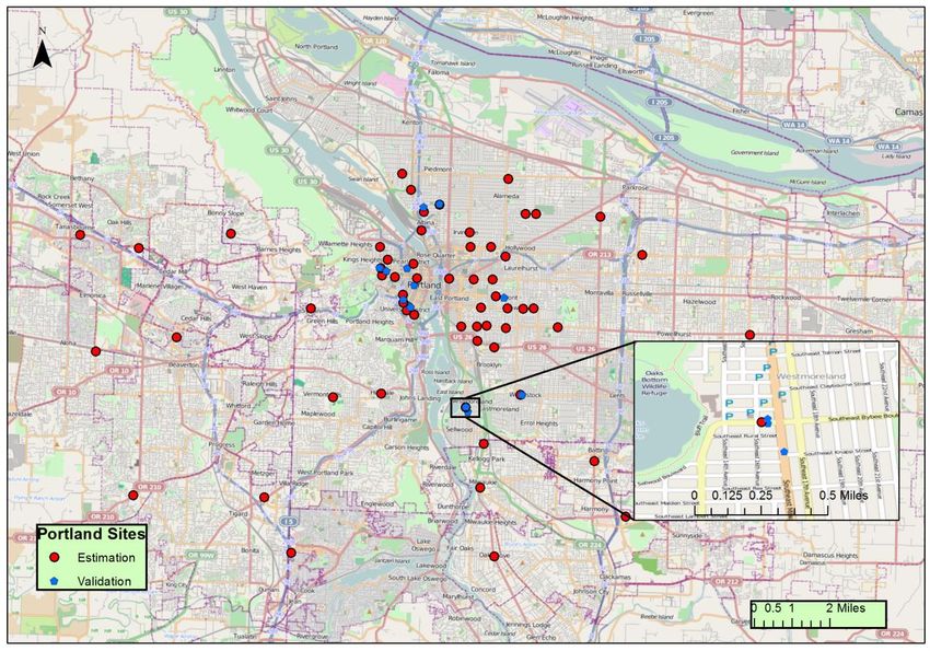
Overview
• Definitions
• Need for adjustments to ITE
• Other adjustment methods
• Development of adjustment
  model in CA                   Image source: Benjamin Sperry

• Considerations & future
  research

                                                         2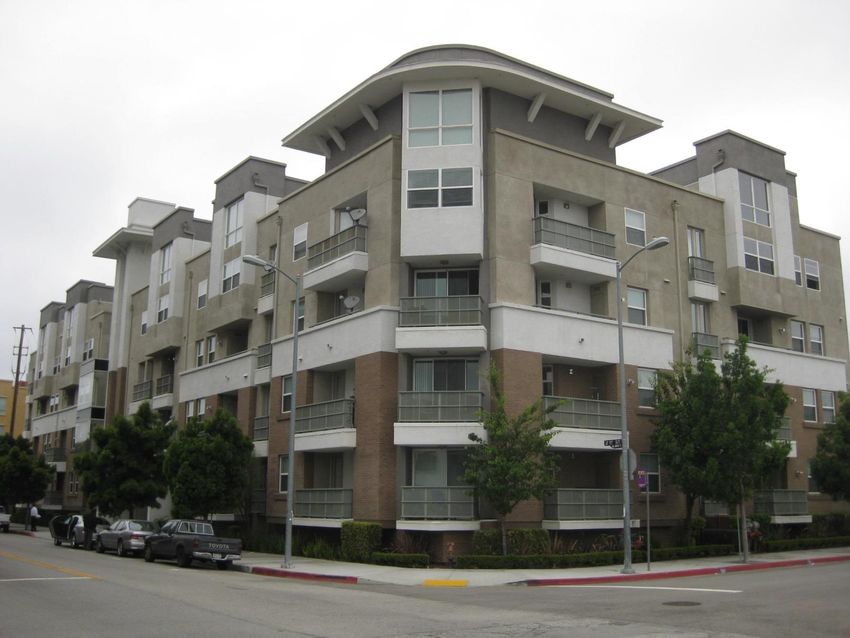
Definitions
• Smart-Growth (SG) Study Site: One of the 65 locations where
  data were collected for this study. Most were individual land
  uses; some MXDs.
• Trip: Movement between a person’s last activity location and the
  targeted use (inbound) or between the targeted land use and
  the next activity location (outbound).

                                                                3
How many vehicle trips are generated
      by a specific land use?

                                       4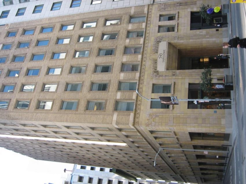
Need for Adjustments to ITE Trip Generation

 • The guidance used most often for
   estimating trip generation is the
   Institute of Transportation
   Engineers (ITE) Trip Generation
   Handbook.

 • California Environmental Quality Act (CEQA),
   requires developers in CA to estimate the
   transportation impacts of proposed
   developments.
                                                  5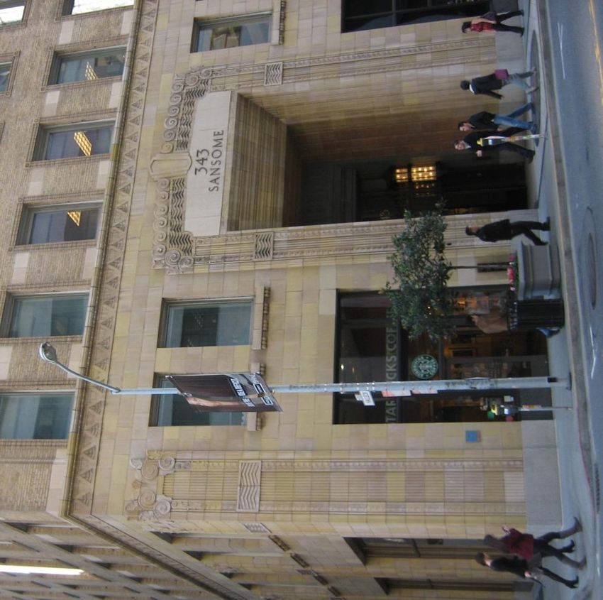
Need for Adjustments to ITE Trip Generation
• Research suggests that vehicle use is generally lower at smart
  growth developments…

Authors (Year)             Study Locations                General Findings
Arrington & Cervero        17 TOD Study Sites              • Weekday trips were 44% lower than ITE
(2008)                     (Philadelphia, Portland, DC,    • AM peak trips were 49% lower than ITE
                           & San Francisco regions)        • PM peak trips were 48% lower than ITE

Kimley Horn & Associates   16 Infill Study Sites          3 mid-rise apartments:
(2009)                     (Los Angeles, San Diego, &      • AM peak trips were 27% lower than ITE
                           San Francisco Regions)          • PM peak trips were 28% lower than ITE
                                                          4 general office buildings:
                                                           • AM peak trips were 50% lower than ITE
                                                           • PM peak trips were 50% lower than ITE
                                                          2 quality restaurants:
                                                           • AM peak trips were 35% lower than ITE
                                                           • PM peak trips were 26% lower than ITE

                                                                                                6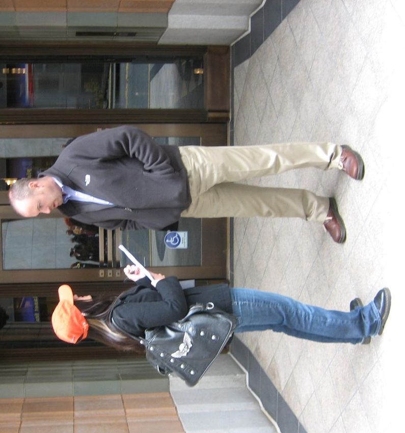
Need for Adjustments to ITE Trip Generation
           ITE-Estimated Vehicle-Trips
    vs. Actual Vehicle-Trips at 30 CA SG Sites

 • On average, ITE-estimates were 2.3 times higher
   than actual vehicle-trips in the AM peak hour
 • On average, ITE-estimates were 2.4 times higher
   than actual vehicle-trips in the PM peak hour

Schneider, R.J., K. Shafizadeh, B.R. Sperry, and S.L. Handy. “Methodology to Gather Multimodal Trip
Generation Data in Smart-Growth Areas,” Transportation Research Record: Journal of the
Transportation Research Board, Volume 2354, pp. 68-85, 2013.                                      7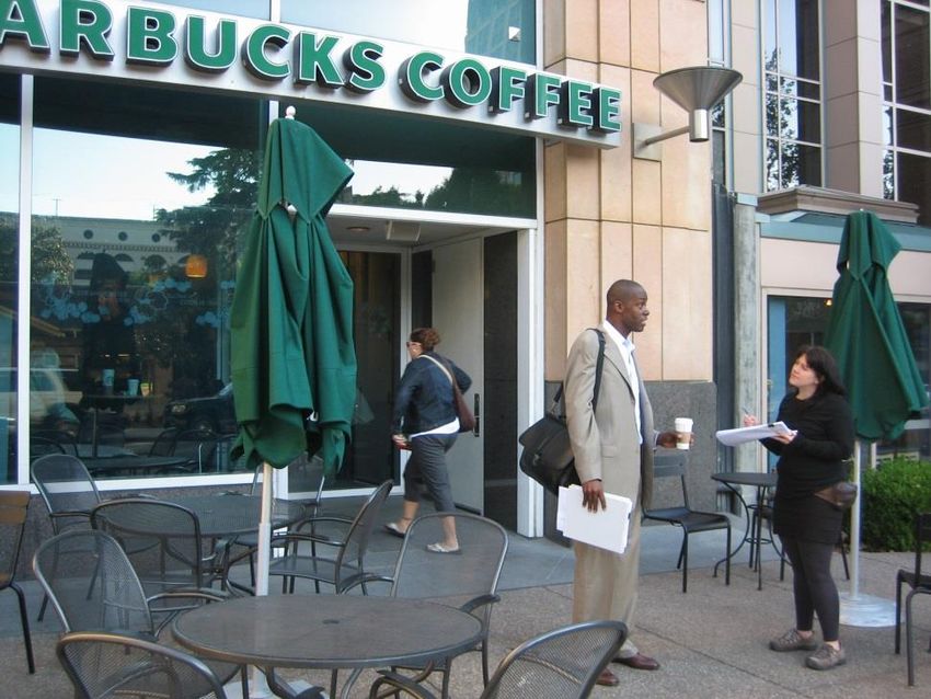
Need for Adjustments to ITE Trip Generation
• Using the ITE Trip Generation methodology on SG
projects likely over-estimates vehicle trips
Mitigation over-emphasizes vehicle needs and
under-supplies transit, pedestrian, & bicycle
facilities
• ITE Trip Generation rates remain widely used in
practice and are based on large amount of data.
How can ITE Trip Generation Estimates be modified
or adjusted for smart growth locations?
8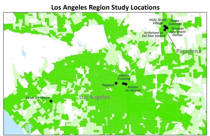
Previous Methods to Adjust ITE
                  Trip Generation Estimates
 •    ITE Multi-Use Method (ITE 2004)
 •    NCHRP 8-51 Method (Bochner et al. 2011)
 •    EPA/SANDAG Method (SANDAG 2010)
 •    URBEMIS Method (Jones & Stokes Associates 2007)
 •    MTC Survey Method (MTC 2006)
 •    San Francisco Method (City and County of SF 2002)
 •    New York City Method (Rizavi and Yeung 2010)

Shafizadeh, K., R. Lee, D. Niemeier, T. Parker, and S. Handy. “Evaluation of Operation and Accuracy of
Available Smart Growth Trip Generation Methodologies for Use in California.” Transportation
Research Record: Journal of the Transportation Research Board, 2307:120-131, 2012.                  9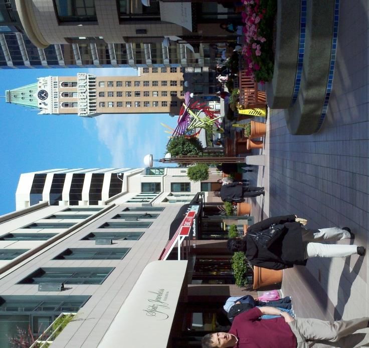
Previous Methods to Adjust ITE
                  Trip Generation Estimates
 • Practical limitations of all methods
       – (e.g., ease of use, sensitivity to SG variables, input
         requirements, output features)
 • All methods performed better than ITE, but no
   method was superior to others (based on 22 sites)
 • SF & NYC methods were not applicable to other areas

Shafizadeh, K., R. Lee, D. Niemeier, T. Parker, and S. Handy. “Evaluation of Operation and Accuracy of
Available Smart Growth Trip Generation Methodologies for Use in California.” Transportation
Research Record: Journal of the Transportation Research Board, 2307:120-131, 2012.                10
Other Methods to Estimate Trip Generation
Recent US efforts:
• Seattle, WA built environment categories—
probability of choosing auto (Clifton et al. 2012)
• Portland, OR intercept surveys at 78 establishments—
linear regression model to adjust ITE (Clifton et al. 2012)
• Household travel survey-based methods—
NCHRP Report 758 (Daisa et al. 2013); (Currans & Clifton 2014)
International methods:
• UK Trip Rate Information Computer System (TRICS)
• New Zealand Trips and Parking Database Bureau
11Would it work to apply a single
adjustment factor to ITE estimates
all Smart Growth sites?
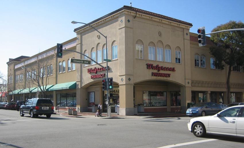
12Example Site 1: 343 Sansome, SF (Office)
13Example Site 2: Park Tower, Sacramento (Coffee)
14Example Site 3: Artisan on 2nd, LA (Residential)
Photo by Ben Sperry, Texas A&M Transportation Institute
15PM Peak Hour Vehicle-Trip Examples
500
450
400
5.8 X
350
300
PM Peak Hour Vehicle-Trips
250
200
150
100
3.5 X
1.4 X
50
0
ITE Actual ITE Actual ITE Actual
343 Sansome, SF Park Tower, Artisan on 2nd, LA
(Office) Sacramento (Coffee) (Residential) 16PM Peak Hour Vehicle-Trip Examples
500
450
400
5.8 X
Study Motivation:
350
What characteristics account
300 for differences in ITE
PM Peak Hour Vehicle-Trips
250 overestimates within
200
Smart Growth areas?
150
100
3.5 X
1.4 X
50
0
ITE Actual ITE Actual ITE Actual
343 Sansome, SF Park Tower, Artisan on 2nd, LA
(Office) Sacramento (Coffee) (Residential) 17Average Discrepancy by LU Category
(CA Smart Growth Sites)
4.0
Average Discrepancy (ITE Vehicle Trips/Actual Vehicle Trips)
3.5
3.0
2.5
ITE Overestimates
2.0
1.5
1.0
ITE Underestimates
0.5
0.0
AM PM AM PM AM PM
(8 Sites) (9 Sites) (4 Sites) (4 Sites) (12 Sites) (11 Sites)
Office Coffee Shop Residential 18A single adjustment factor may not be
appropriate for all Smart Growth sites…
• ITE-estimates were 2.3 to 2.4 times higher than
actual vehicle-trips (on average)
• Evidence of differences by land use category…
– Office: ITE was 2.9 times higher in AM and 3.2 times higher in PM
– Residential: ITE was 1.1 times higher in AM and 1.4 times higher in PM
– Coffee: ITE was 2.6 times higher in AM and 1.2 times higher in PM
Schneider, R.J., K. Shafizadeh, B.R. Sperry, and S.L. Handy. “Methodology to Gather Multimodal Trip
Generation Data in Smart-Growth Areas,” Transportation Research Record: Journal of the
Transportation Research Board, Forthcoming, 2013. 19A single adjustment factor may not be
appropriate for all Smart Growth sites…
• ITE-estimates were 2.3 to 2.4 times higher than
actual vehicle-trips (on average)
• Evidence of differences by land use category…
– Office: ITE was 2.9 times higher in AM and 3.2 times higher in PM
– Residential: ITE was 1.1 times higher in AM and 1.4 times higher in PM
– Coffee: ITE was 2.6 times higher in AM and 1.2 times higher in PM
• Differences by Smart Growth characteristics?…
Schneider, R.J., K. Shafizadeh, B.R. Sperry, and S.L. Handy. “Methodology to Gather Multimodal Trip
Generation Data in Smart-Growth Areas,” Transportation Research Record: Journal of the
Transportation Research Board, Forthcoming, 2013. 20Development of California Smart-Growth
Trip Generation Model
21Criteria for Smart Growth Model Application Smart Growth Criteria • Mostly developed within 0.5 miles of site • Mix of land uses within 0.25 miles of site • Minimum jobs and population within 0.5 miles of site: J>4,000 and R>(6,900-0.1J) Land Use Classification Criteria • Mid- to High Density Residential (ITE Codes 220, 222, 223, 230, 232) • Office (710) • Restaurant (931, 939) • Coffee/donut shop (936) • Retail (820, 867, 880) Transportation System Criteria • Minimum number of bus or transit lines • Bicycle facilities or sidewalk coverage 22
Sites Used for Model Development
         (Los Angeles, San Diego, San Francisco, and Sacramento Regions)

                                                      AM Model                                   PM Model

Residential Land Use                                        20                                         20

Office Land Use                                             11                                         12

Coffee/Donut Land Use                                        3                                          3

MXD Land Use                                                11                                         11

Retail Land Use                                              0                                          3

Other Land Use                                               1                                          1

Total Sites                                                 46                                         50
Sources: 1) EPA MXD Study (2010), 2) SANDAG MXD Study, (2010) 3) Caltrans Infill Study (2009), 4) TCRP Report 128 (2008),
5) Fehr & Peers (2010), 6) UC Davis Team field data collection (2012)
                                                                                                                            23
Model Development: Dependent Variable
actual veh trips
ln
ITE estimated veh trips
24Explanatory Variables
• Land use classification (e.g., office, coffee/donut shop)
• Site characteristics (e.g., off-street surface parking, building setback)
• Adjacent street characteristics
(e.g., number of lanes; pedestrian and bicycle facilities)
• Surrounding area characteristics
(e.g., population & employment density, neighborhood socioeconomics)
• Proximity characteristics
(e.g., distance to transit, distance to retail, distance to university campuses)
25First Tried One-Step Linear Regression Model
• Attempted to identify singular variables most
strongly associated with reduced trips
• Challenge: many SG variables are highly correlated
(e.g., high employment density, less off-street parking,
metered on-street parking & more transit service)
• It is likely that many SG variables are working
together collectively to influence mode choice
26Decided on Two-Step Approach:
Factor Analysis then Linear Regression Model
Factor Analysis
• Identifies smart growth
variables that may be
“working together”
• Quantifies the
cumulative impact of
this set of variables
27Factor Analysis:
Smart Growth Factor
Variable Coefficient*
Population within 0.5 miles (000s) 0.099
Jobs within 0.5 miles (000s) 0.324
Distance to center of CBD (in miles) -0.138
Average building setback from sidewalk -0.167
Metered parking within 0.1 miles (1=yes, 0 = no) 0.184
Number of bus lines within 0.25 miles 0.227
Number of rail lines within 0.5 miles 0.053
Percent of site area covered by surface parking -0.080
*This coefficient is applied to the standardized version of the variable which is calculated by subtracting the
mean and dividing by the standard deviation from the 50 PM analysis sites.
28Linear Regression:
Final AM and PM Peak Hour Models
Dependent Variable = Natural Logarithm of Ratio of Actual Peak Hour Vehicle Trips to ITE-Estimated
Peak Hour Vehicle Trips
AM Model PM Model
Coeff. t-value p-value Coeff. t-value p-value
Smart Growth Factor -0.096 -0.857 0.397 -0.155 -1.491 0.143
Office land use (1 = yes, 0 = no) -0.728 -3.182 0.003 -0.529 -2.558 0.014
Coffee shop land use (1 = yes, 0 = no) -0.617 -1.677 0.101 -0.744 -2.339 0.024
Mixed-use development (1 = yes, 0 = no) -0.364 -1.561 0.127 -0.079 -0.381 0.705
Within 1 mi. of university (1 = yes, 0 = no) -1.002 -2.285 0.028 -0.311 -1.099 0.278
Constant -0.304 -2.460 0.018 -0.491 -4.469 0.000
Overall Model
Sample Size (N) 46 50
Adjusted R2-Value 0.294 0.290
F-Value (Test value) 4.74 (p = 0.002) 4.99 (p = 0.001)
29Linear Regression:
Final AM and PM Peak Hour Models
Dependent Variable = Natural Logarithm of Ratio of Actual Peak Hour Vehicle Trips to ITE-Estimated
Peak Hour Vehicle Trips
AM Model PM Model
Coeff. t-value p-value Coeff. t-value p-value
Smart Growth Factor -0.096 -0.857 0.397 -0.155 -1.491 0.143
Office land use (1 = yes, 0 = no) -0.728 -3.182 0.003 -0.529 -2.558 0.014
Coffee shop land use (1 = yes, 0 = no) -0.617 -1.677 0.101 -0.744 -2.339 0.024
Mixed-use development (1 = yes, 0 = no) -0.364 -1.561 0.127 -0.079 -0.381 0.705
Within 1 mi. of university (1 = yes, 0 = no) -1.002 -2.285 0.028 -0.311 -1.099 0.278
Constant -0.304 -2.460 0.018 -0.491 -4.469 0.000
Overall Model
Sample Size (N) 46 50
Adjusted R2-Value 0.294 0.290
F-Value (Test value) 4.74 (p = 0.002) 4.99 (p = 0.001)
30Linear Regression:
Final AM and PM Peak Hour Models
Dependent Variable = Natural Logarithm of Ratio of Actual Peak Hour Vehicle Trips to ITE-Estimated
Peak Hour Vehicle Trips
AM Model PM Model
Coeff. t-value p-value Coeff. t-value p-value
Smart Growth Factor -0.096 -0.857 0.397 -0.155 -1.491 0.143
Office land use (1 = yes, 0 = no) -0.728 -3.182 0.003 -0.529 -2.558 0.014
Coffee shop land use (1 = yes, 0 = no) -0.617 -1.677 0.101 -0.744 -2.339 0.024
Mixed-use development (1 = yes, 0 = no) -0.364 -1.561 0.127 -0.079 -0.381 0.705
Within 1 mi. of university (1 = yes, 0 = no) -1.002 -2.285 0.028 -0.311 -1.099 0.278
Constant -0.304 -2.460 0.018 -0.491 -4.469 0.000
Overall Model
Sample Size (N) 46 50
Adjusted R2-Value 0.294 0.290
F-Value (Test value) 4.74 (p = 0.002) 4.99 (p = 0.001)
Bold values indicate p-values < 0.15 31High & Low Examples (PM Model)
• Office project with highest value SGF in sample = 2.41
– Ratio actual/ITE-estimated is 0.248
– 75% vehicle trip reduction from ITE
• Office project with lowest value SGF in sample = -1.44
– Ratio actual/ITE-estimated is 0.451
– 55% vehicle trip reduction from ITE
• Residential project with lowest value SGF in sample = -1.44
– Ratio actual/ITE-estimated is 0.765
– 23% vehicle trip reduction from ITE
32PM Model Validation (N = 13)
33PM Model Validation (N = 13)
34Sneak Preview: Model Verification
How well does the PM model
work at a sample of sites in a
different urban region?
Portland, OR
35Model Verification
Observed versus Predicted
Ratios to ITE Estimates:
20 Most Appropriate
Portland Sites
Image Source: Andrew McFadden, UC Davis 36Model Verification
ITE- and Model-
Estimated Trips vs.
Actual Trips:
20 Most Appropriate
Portland Sites
Image Source: Andrew McFadden, UC Davis 37Modeling Considerations
• Small sample size (N=46; N=50)
• Considered variables for LU mix; residential LU
• MXD sites (not used in model application)
• Did not account for some variation
– e.g., Economic activity, attitudes
38Model Development: Big Picture
• Final models balance theory and practice
• Complement existing ITE Trip Generation method
• Two-step method was a key breakthrough
39Spreadsheet Tool
Downtown LA Example:
72% vehicle trip reduction
from ITE during PM peak
40Future Research: Outstanding
Transportation Impact Assessment Issues
• Should we use existing ITE Trip Generation Manual
data (isolated, suburban site database) as a basis for
SG adjustments?
• Model multimodal person trips
• Measuring impact: number of trips vs. trip length
41Acknowledgements
• California Department of Transportation
– Terry Parker, Project Manager
– Practitioner Panel
• Data collection team members
– Ewald & Wasserman Research Consultants
– Gene Bregman & Associates
– Manpower
• Data entry and Q/C team members
– Calvin Thigpen, UC Davis
– Mary Madison Campbell, UC Davis
• Data collection methodology
– Brian Bochner, TTI
– Ben Sperry, TTI
• Property managers and developers Image source: Benjamin Sperry
For more information, see project website:
http://ultrans.its.ucdavis.edu/projects/smart-growth-trip-generation
42Questions & Discussion
For more information, see the project website:
http://ultrans.its.ucdavis.edu/projects/
smart-growth-trip-generation
43Factor Analysis: Smart Growth Factor
• Based on data from 50 PM sites
• Principal Axis Factoring (accommodates variables
that are not normally-distributed)
• The single Smart Growth Factor (SGF) explained
49.5% of the variation in the data, while the second
factor only explained 17.3% of the variation
• The ratio of the sample size and the number of
variables included in the SGF is 50/8 = 6.25/1. This
is similar to many studies reviewed in Costello and
Osborne (2005).
Useful Reference: Costello, A.B. and J.W. Osborne. “Best Practices in Exploratory Factor Analysis:
Four Recommendations for Getting the Most from Your Analysis,” Practical Assessment, Research
44
and Evaluation, 10(7). Available online: http://pareonline.net/getvn.asp?v=10&n=7, 2005.Factor Analysis: Smart Growth Factor Loadings
Variable Loading
Population within 0.5 miles (000s) .538
Jobs within 0.5 miles (000s) .781
Distance to center of CBD (in miles) -.632
Average building setback from sidewalk -.636
Metered parking within 0.1 miles (1=yes, 0 = no) .707
Number of bus lines within 0.25 miles .745
Number of rail lines within 0.5 miles .661
Percent of site area covered by surface parking -.467
45San Francisco Region Study Sites
46Los Angeles Region Study Sites
47Sacramento Region Study Sites
48Future Research: Model Improvement
• More data to refine models; test in other regions
• Need SG adjustments for more land uses
4978 Sites in Portland, OR Data Source: Clifton, et al., Portland State University, 2012. Image Source: Andrew McFadden, UC Davis 50
Model Verification

Observed versus Predicted
 Ratios to ITE Estimates:
       All 78 Sites

    Image Source: Andrew McFadden, UC Davis   51
You can also read


