MOHO TOPOGRAPHY AND VELOCITY/DENSITY MODEL FOR THE HEDMARKEN AREA, EASTERN NORWAY, USING RECEIVER FUNCTION ANALYSIS AND RJ-MCMC - CLAUDIA PAVEZ ...
←
→
Page content transcription
If your browser does not render page correctly, please read the page content below
Moho Topography and Velocity/Density Model
for the Hedmarken area, Eastern Norway, using
       Receiver Function Analysis and Rj-McMC
     Claudia Pavez, Marco Brönner, Arne Bjørlykke, Odleiv Olesen
     Geological Survey of Norway

                                                                   © Authors. All rights reserved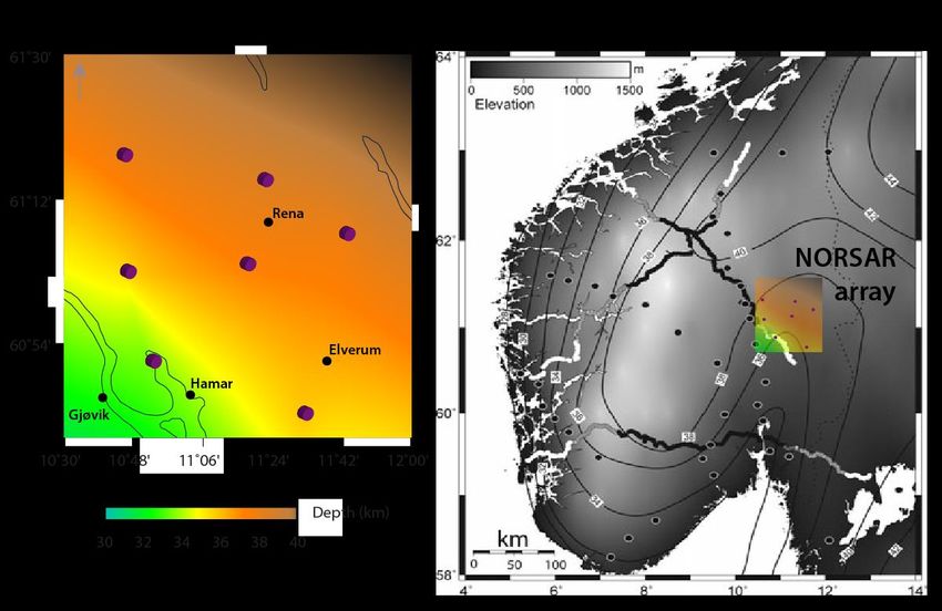
To follow this presentation
This slide explains how to understand the presentation through the methodological
sequence. In the upper right corner of each slide you will find the number that is
corresponding to the specific methodologies listed below

                   VISUALIZATION &                                     METHODOLOGY
                   GEOPGRAPHIC INFORMATION
                   SYSTEMS                                             Seismic processing:

                   0. GMT                                              1. IRIS Wilber3
                      QGIS                                             2. SAC

                                                                       Transdimensional inversion

                                                                       3. Rj-rf
                                                                       4. Rj-McMC
                                                                       (Reversible jump receiver
                                                                       function & Reversible jum
                                                                       Markov chain Monte Carlo)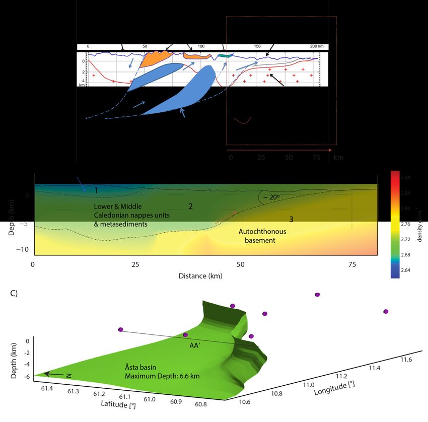
0
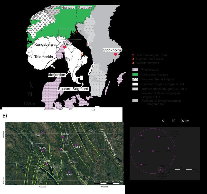
Study area: Central-Eastern Norway, Hedmarken
Table 1: NORSAR large aperture seismic array
Station Latitude Longitude Elevation
code [°] [°] [m]
NAO01 60.844 10.886 426
NBO00 61.030 10.777 529
NC204 61.275 10.762 851
NC602 60.735 11.541 305
NB201 61.049 11.293 613
NC405 61.112 11.715 496
NC303 61.225 11.369 401
Figure 1: A). Sketch map showing the lithotectonic units of the Sveconorwegian Orogenic Belt (Modified from Bingen & Viola,
2018). The black box is showing the location of the NORSAR array and the interpolation area used in this research B). Digital Pavez et al., 2020.
elevation model showing a zoom-in of the seismic stations. Green lines correspond to the major faults observed in the zone,
mainly composed by NS and NNW lineaments near to the array. Dotted green line delineates the Sveconorwegian front. C).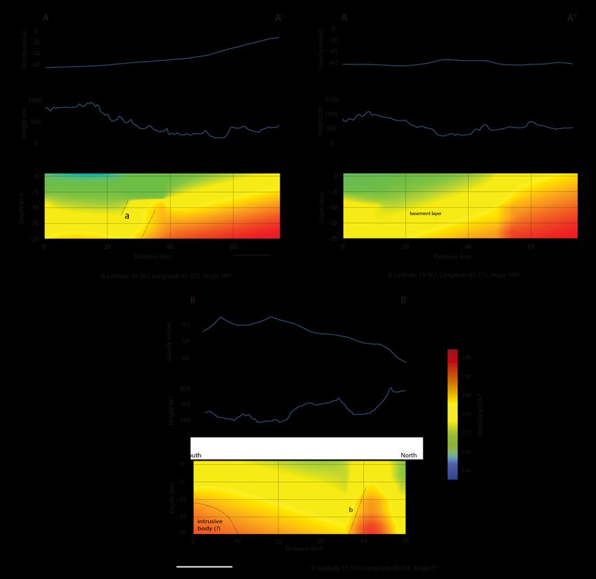
Part I:
HK Stacking

              Figure from C. Ammon’s receiver function webpage
              (see references)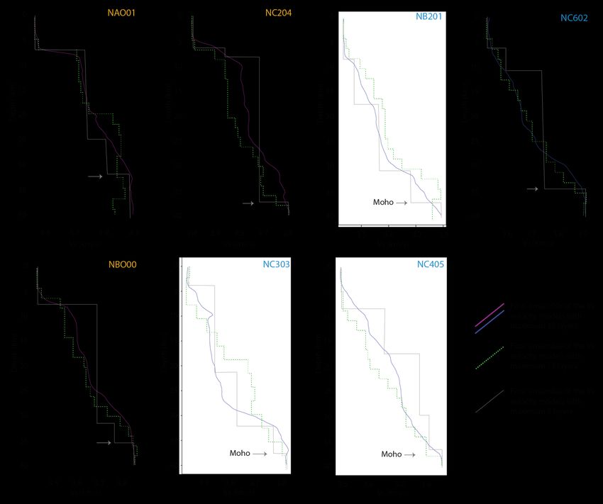
0
Recorded teleseismicity                                                                                              1

• We used 50 teleseismic events
recorded during the 2017-2018
period by the NORSAR array.

• A set of 20 high magnitude events
(Mw ≥ 6.0, Mb ≥ 5.6) with epicentral
distances between 30° - 90° was
selected according quality.

• The ray parameter (p) was calculated
 per each event.

   Figure 2: Location of teleseismic events accepted for processing and stacking (red stars). All   Pavez et al., 2020.
   the events are located between 30° - 90° from the study area, centered at NB201 seismic
   station (blue triangle) (from Pavez et al., 2020)
Receiver functions                                 2

The receiver functions were
calculated through time-
domain deconvolution , using
the CPS seismology package
(Ligorria & Ammon, 1999;
Hermann, 2013)

Figure 3: Stacked & non-scaled
receiver functions for each
seismic station. The main
phases are shown and the intra-
crustal discontinuities related
to the Åsta basin are marked
with a green arrow.

                                  Pavez et al., 2020.
HK Stacking results 2
Station H (km) ĸ Poisson’s ratio
NAO01 33.5 0.31 1.72 0.015 0.245
According to the receiver functions NBO00 35.3 0.30 1.71 0.02 0.240
and the arrival times of the different NC204 37.8 0.31 1.76 0.015 0.262
phases (P and Ps), the HK stacking NC602 35.9 0.40 1.78 0.05 0.269
method was applied. NB201 37.1 0.31 1.73 0.01 0.249
NC405 37.8 0.67 1.79 0.09 0.273
NC303 38.4 0.31 1.71 0.02 0.240
Table 2: HK Stacking results per station, including projected
errors. The western cluster is shown in orange and the eastern
one in blue.
Pavez et al., 2020.Mohorovicic depth: 2D projection 0
Figure 4: A. Local crustal
thickness beneath the
NORSAR network. Purple
circles correspond to the
location of seismic stations.
B. Original Moho map for
Southern Norway proposed
by Stratford et el., (2009).
The original image was
modified overlapping the
results obtained in this
research for comparative
purposes.
Pavez et al., 2020.3
4
Part II:
Transdimensional
inversion
Figure 5: Schematic representation of a one-dimensional transdimensional model applied
to receiver function inversion. mi represents the velocity, which is the model unknown,
but additionally the number of layers and their thicknesses are also a variable.
Figure modified from Sambridge et al., 20133
Velocity models 4
The velocity models were calculated
using the receiver functions and the Rj-rf
code available at the iEarth webpage
(see references). The input parameters
can be observed in Table 3:
Number of 80000
iterations
Burn-in period 10000 iterations
Depth 0 – 40 km
Vs 3.30 – 4.50 km/s
Maximum number 35, 15, 5 for models
of partitions 1, 2 and 3,
(layers) respectively
Figure 6: Posterior ensemble showing
the 1D S- wave velocity model for all
stations. The seismic stations
belonging to the western cluster are
shown with an orange legend. Seismic
stations corresponding to the eastern
part, are shown with a light blue
legend.
Pavez et al., 2020.3
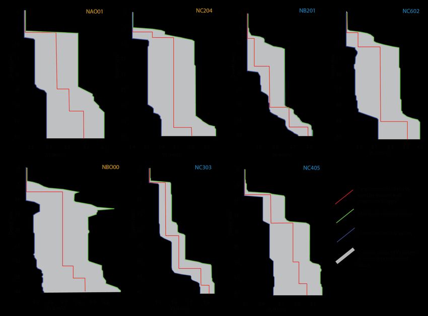
2D/3D density model 4
Figure 7: 1D S-wave velocity
models delimiting the model
space for all seismic stations.
The gray shaded area shows
the entire sampled model
space. The colored lines
represent the minimum
credible values, the ensemble
solution and the maximum
credible values in blue, red and
green, respectively.
Pavez et al., 2020.2D/3D density model 0
Figure 8: A,B & C
correspond to the density
models for the AA’, AA’’ and
BB’ cross sections.
Additionally, topography
and observed gravity are
shown. Inferred thrust faults Applying the Nafe-Drake curve,
are marked with dotted we obtained a velocity model from
lines. All profiles are using the Vp values.
the same color palette. It is possible to infer most
likely NW dipping ENE-WSW
striking major Normal faults in
the Precambrian basement, which
marks the tectonic boundary of
the basin
Pavez et al., 2020.2D/3D 0
density model
Figure 9: A. Geological cross
section presented by Bjørlykke
& Olesen (2018). Red dotted
box is showing the subsection
where the profile is compared
with the AA’ density model.
B. Density model for the AA’
cross section, including the
interpretation according to A).
C. 3D model showing the
outline shape of the Åsta Basin.
Purple dots correspond to the
seismic network and position of
the AA’ profile is shown as a
continuous black line.
Pavez et al., 2020.Main references and funding source
Ammon, C. 1997. Personal webpage receiver function subsection
http://eqseis.geosc.psu.edu/cammon/HTML/RftnDocs/rftn01.html
This project was funded by the Bjørlykke, A. & Olesen, O. 2018: Caledonian deformation of the Precambrian basement in southeastern Norway. Norwegian
Chilean state through the Journal of Geology 98, 1–16.
Postdoctoral fellowship Bodin, T., Sambridge, M., Tkalčić, H., Arroucau, P., Gallagher, K. & Rawlinson, N. 2012: Transdimensional inversion of receiver
functions and surface wave dispersion. J. Geophys. Res., 117, B02301. doi:10.1029/2011JB008560.
‘Postdoctorado en el extranjero
Becas Chile 2019’ project number Hermann, R. 2013: Computer Programs in Seismology: An evolving tool for instruction and research. Seismological Research
Letters 84. 1081–1088.
74200005 ‘Seismic Imaging using
Norwegian Earthquakes’. IEarth free software Rj-rf. http://www.iearth.org.au/codes/rj-RF/.
Ligorria, J.P., Ammon, CJ. 1999: Iterative deconvolution and receiver-function estimation. Bulletin of Seismological Society of
Additionally, this research was America 89 (5). 1395–1400.
possible thanks to the support of Pavez, C., Brönner, M., Bjørlykke, A., Olesen, O. 2020: Moho topography and velocity /density model for the Hedmarken area,
the Geological Survey of Norway Eastern Norway. NGU report 2020.013. 43 pp.
(NGU). The authors are also Sambridge, M., Bodin, T., Gallagher, K., Tkalčić, H. 2013: Trans-dimensional inference in the geosciences, Phil. Trans. R. Soc. A,
grateful for the IRIS Data Center 371, 20110547. doi:10.1098/rsta.2011.0547.
freely providing the data applied Stratford, W., Thybo, H., Faleide, J.I., Olesen, O., Tryggvason, S. 2009: New Moho map for onshore southern Norway.
for this research study. Geophysical Journal International 178, 1755–1765.
Zhu, L. & H. Kanamori. 2000: Moho depth variation in southern California from teleseismic receiver functions. Journal of
Geophysical Research, 105, 2969–2980.
© Authors. All rights reservedYou can also read