Modelling Collie power stations with TAPM - Ken Rayner Department of Environment and Conservation, Western Australia
←
→
Page content transcription
If your browser does not render page correctly, please read the page content below
Modelling Collie power stations
         with TAPM

             Ken Rayner
    Department of Environment and
    Conservation, Western Australia
           September 2009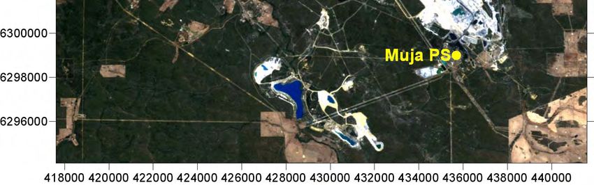
Background
• Collie is ~ 150 km SSW of Perth
• existing and proposed coal fired power
  stations within the basin
• other industries proposed for the basin
• potential air quality concerns, notably SO2
  and particulates
Bluewaters
Bluewaters PS
Power
stations Collie PS
and
monitoring
sites Collie Shotts
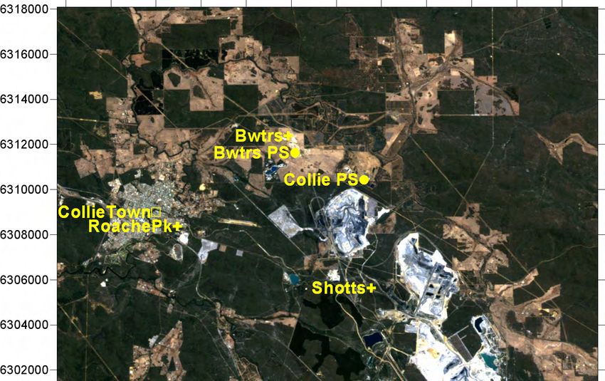
Muja PS
10 km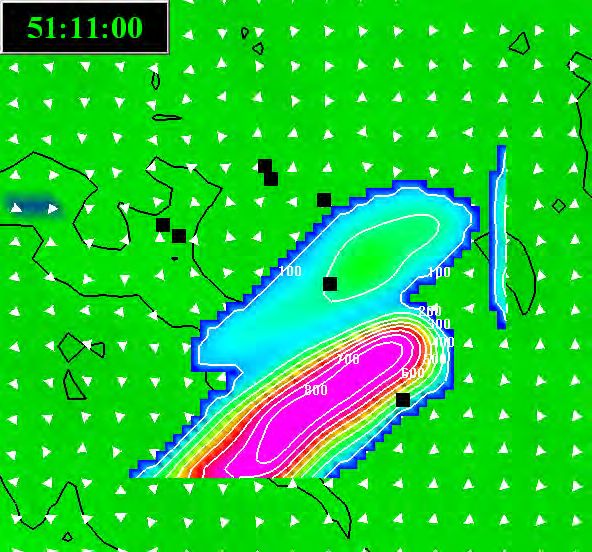
Air quality studies and TAPM
• (selective summary for purposes of this talk)
• monitoring program 1995‐2002 (SO2, met)
• Hibberd and Physick (2003) (H&P)
  – data analysis
  – TAPM 2.0 testing, recommended parameters
• EIA projects 2004 – 2009 based on H&P, using
  various versions of TAPM for 2001 met
Hibberd and Physick (2003) (H&P)
• hourly emissions data
• analysis of met and SO2 data ‐ dominant process was
  strongly convective conditions:
   – morning inversion break‐up with fumigation
   – late morning to afternoon convective mixing with plume
     ground‐strikes.
• TAPM tests to choose values for plume buoyancy
  enhancement factors and surface roughness
• monthly deep soil moisture values recommended
• Eulerian dispersion for all sources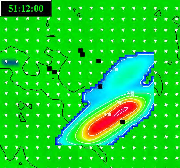
Collie

Hibberd,
Physick and
Park
(CASANZ        Shotts
2003)
all Eulerian

               Bluewaters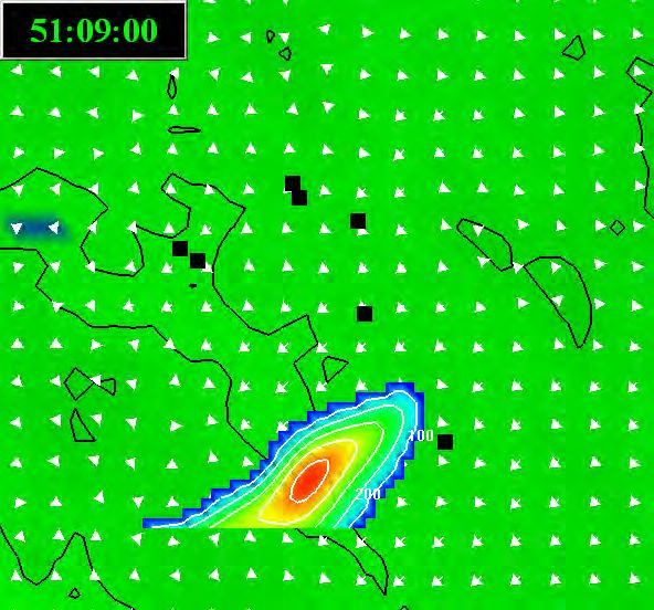
Hibberd and Physick conclusions
• good data set
• based on statistical analysis of results for
  three years, the third highest TAPM prediction
  provides a good estimate of the maximum
  observed concentrations
DEC concerns
• EIA studies since 2003 have used evolving
  TAPM versions and different mixtures of
  Eulerian / Lagrangian dispersion while
  retaining H&P moisture, plume buoyancy;
• Apparent tendency to increased over‐
  estimation of concentrations (exacerbating
  tendency seen in H&P)
• Loss of comparability to original H&P
TAPM grid for all modelling
Meteorology
  35 x 35 x 25 grid points
  30, 10, 3, 1 km spacing
Air quality
  15, 5, 1.5, 0.5 km spacing
Muja
reasonably
clear of grid
boundaries
Purpose of this investigation
Consider relative differences due to:
– model version change
– Eulerian (E) vs. Lagrangian (L) dispersion
while holding other model parameters
unchanged.
Note: TAPM 4 runs will use all recommended
options, including V4 land use scheme. Hence
soil moisture different.
TAPM bug
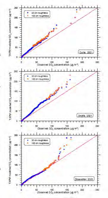
Collie
monitoring
station.

Reproduction
of Hibberd and
Physick (2003)

- Eulerian
Shotts
monitoring
station.

Reproduction
of Hibberd and
Physick (2003)

- Eulerian
Bluewaters
monitoring
station.

Reproduction
of Hibberd and
Physick (2003)

- Eulerian
Collie
monitoring
station.

Comparing
TAPM
versions

- Eulerian
Shotts
monitoring
station.

Comparing
TAPM
versions

- Eulerian
Bluewaters
monitoring
station.

Comparing
TAPM
versions

- Eulerian
Collie
monitoring
station.

Comparing
TAPM
versions

- Lagrangian
(except Worsley
Shotts
monitoring
station.

Comparing
TAPM
versions

- Lagrangian
(except Worsley
Bluewaters
monitoring
station.

Comparing
TAPM
versions

- Lagrangian
(except Worsley
Summary
• significantly greater over‐estimation in TAPM
  3.0.7 and 4.0 results relative to TAPM 2.0, for
  both E and L dispersion
• does not necessarily mean TAPM performance
  has degraded. (e.g. HP “tuned” Muja plume
  buoyancy parameters using TAPM 2 in E
  mode). CSIRO’s TAPM tests do not suggest
  consistent over‐estimation for 3.0.7, 4.0
• changing from Eulerian (E) to Lagrangian (L)
  dispersion produces some interesting results
Shotts
monitoring
station.

Comparing
E vs L
dispersion

- TAPM 3.0.7
Collie
monitoring
station.

Comparing
E vs L
dispersion

- TAPM 3.0.7
High E values dominated by
               Muja which is 17 km from Collie
Collie
monitoring
station.

Comparing
E vs L
dispersion
Muja PS – E
Collie A – L

- TAPM 3.0.7
Collie monitoring station. Comparing E vs L dispersion - daytime - TAPM 3.0.7
Collie
monitoring
station.

Comparing
E vs L
dispersion
- night-time

- TAPM 3.0.7
Summary E results significantly over‐estimate observations at both sites, both day and night; L results are similar to E results during daytime, but are significantly lower than E and closer to observations during night‐time. Same day / night pattern for Shotts. Isn’t daytime when we would expect L and E to differ most? Other explanation?
Summary cont...
• Some folks think that Lagrangian modelling is
  not required if the receptors of interest are
  beyond 900 sec travel time (after the hybrid
  LPM mode has switched to the EGM).
  – i.e. “Eulerian dispersion will give the same results
    as Lagrangian at distant receptors.”
• NOT CORRECT.
Wind speed for top 30 concentrations at Collie
in 2001 (Eulerian and Lagrangian) - Night only
300
Concentration ( μ g/m )
3
250
Eulerian mostly < 4 m/sec. Travel
time > 4000 sec (>> 900 sec).
Lagrangian does not produce
200
matching results for low speed /
long travel times. CO TAPM 307 E
150
CO TAPM 307 L
100
50 17 km in
Every L has switched to E 900 sec
0
0 2 4 6 8 10 12 14 16 18 20
Wind speed at 150 metresCSIRO advice • Because the initial dispersion is different in the two modes, results can be different further downwind, even after the hybrid LPM mode has switched to the EGM mode. • we (CSIRO) recommend LPM for all point sources because we consider that this provides the better physical description of point source plume dispersion.
Uncertainty in extreme event
        predictions
Bluewaters
Bluewaters PS
Power
stations Collie PS
and
monitoring
sites Collie Shotts
Muja PS
10 kmTAPM 3.0.7 Max 1-hr SO2 Collie too close to grid boundary
TAPM 3.0.7
Max 1-hr
SO2
Met grid
shifted W
slightly,
pollution grid
slightly
expanded.
Significant
changes
TAPM 3.0.7
9th highest
SO2
Collie too
close to grid
boundary
TAPM 3.0.7
9th highest
SO2
Grid shifted W
& expanded
slightly.

No major
changes
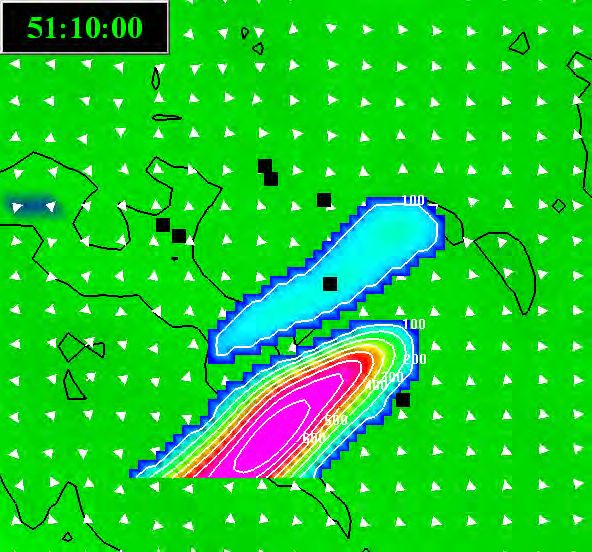
TAPM 3.0.7
Max 1-hr
SO2

Examine this
“sausage
TAPM 3.0.7
Max 1-hr
SO2
Muja C&D
20 Aug only
11:00 peak
concentration
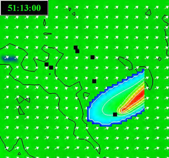
u < 1m/sConcentration profiles on 20 Aug 2001 at location
of highest 1-hour maximum from Muja PS
TAPM 3.0.7 600
Muja C&D
500
20 Aug
8:00 - 12:00 400
Height (m)
12:00
plume 300
11:00
10:00
fumigation 9:00
within 8:00
200
growing
mixed layer 100
0
0 500 1000 1500 2000 2500 3000 3500
Concentration (ug/m3)TAPM 3.0.7 Muja C&D 20 Aug u @ 250 m plume fumigation within growing mixed layer
TAPM 3.0.7
Muja C&D
20 Aug
u @ 250 m
plume
fumigation
within
growing
mixed layer
TAPM 3.0.7
Muja C&D
20 Aug
u @ 250 m
plume
fumigation
within
growing
mixed layer
TAPM 3.0.7
Muja C&D
20 Aug
u @ 250 m
plume
fumigation
within
growing
mixed layer
TAPM 3.0.7
Muja C&D
20 Aug
u @ 250 m
plume
fumigation
within
growing
mixed layer
TAPM 3.0.7
Muja C&D
20 Aug
u @ 250 m
plume
fumigation
within
growing
mixed layer
Summary
• this “sausage” is caused by a credible
  fumigation event (analyses of wind and
  temperature profiles adds support).
• But how much reliance should be placed on
  the prediction of this event (or similar events),
  noting that it appeared due to an innocuous
  change of grid centre and slight grid
  expansion?
Sensitivity tests
The sausage reduced markedly in magnitude or
  disappeared when:
• the grid was moved further south;
• model was started on 18 and 16 August (2 and
  4 spin‐up days)
Also sensitive to the number of sources (which
  slightly affects meteorology – compiler
  optimisation issue?)
TAPM 3.0.7
Max 1-hr
SO2
+Muja A and B

Enhanced
sausage
TAPM 3.0.7
Max 1-hr
SO2
+Muja A and B
+3 very small
sources
Sausage has
vanished,
other
variations
apparent
• variation also evident in TAPM 4 max
• 9th highest hour results much less sensitive to
  model configuration changes than max hour.
• strong argument to use 9th highest hour (or
  similar) as a stable model statistic for
  assessment purposes.
• BUT you then need an assessment criterion
  for the 9th highest hour.
NZ modelling guide (2004)

99.9% value reported must be with reference to a specific receptor
• amounts to saying “model are always
  seriously biased high – concentrations are
  always significantly over‐estimated across the
  distribution of concentrations (not just the
  maximum)”
• incorrect – not true in general
• a skilful model does not exhibit uniform bias –
  plenty of examples.
TAPM 4 ‐ Kincaid (Hurley et al., 2008)
Aermod Kincaid (Paine et al., 1998)

2.1

                                  4.0
TAPM and DISPMOD re Kwinana
(Hurley et al., 2005)
measured
measured
99.9% 99.9%
Model matches measured very well at 99.9 percentile. Max
and RHC of measured are much higher than 99.9 percentile
at both sites.• for point sources, the 9th highest glc is typically 50 to 75% of the max glc at any given impacted location. • if using an unbiased model, the 9th highest prediction would be a serious underestimate of the actual highest (or second highest). • Kwinana: 350 μg/m3 99.9% is similar in stringency to the NEPM 570 μg/m3 2nd highest.
Recommendation
• Don’t confuse the need for a stable model
  statistic with model bias.
• Use something like 99.9 percentile 1‐hour
  average as a stable statistic for assessment
  against a 99.9 percentile 1‐hour criterion.
• Correction of known model bias should be
  case‐by‐case via a clearly explained empirical
  fix. Might involve a case‐specific (not
  generally applicable) use of a different
  percentile,
• and if your model is always biased, perhaps it
  is time to fix it or get a new model.
You can also read