Scattering of a Plane EM Wave on a PEC Infinite Cylinder - Department of Microelectronics and Computer Science Technical University of Lodz ...

Department of Microelectronics and Computer Science
                Technical University of Lodz

   Scattering of a Plane EM
    Wave on a PEC Infinite
           Cylinder

M.Sc. Marta Zawieja
zawiejam@dmcs.p.lodz.pl

                          Lodz, August 2002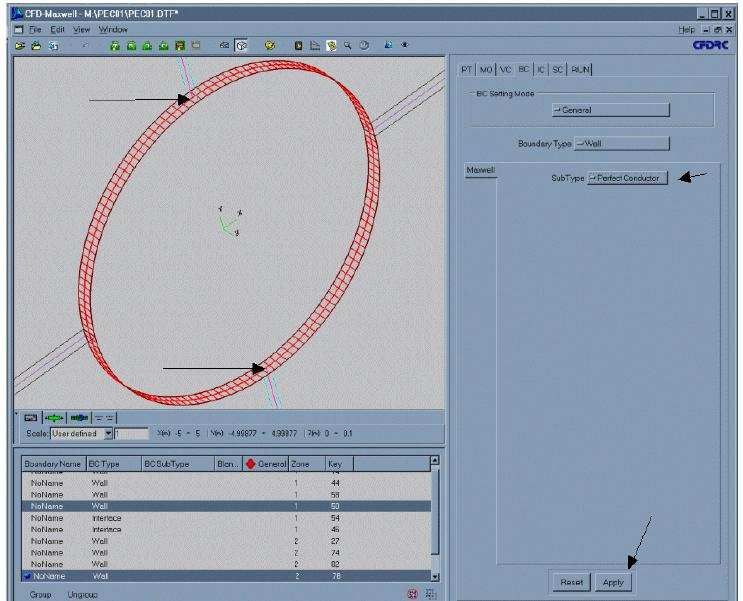

Problem description:

The interconnects and the devices formed by interconnects such as inductors,
filters, resonant circuits, transformers and antennas are very often used in the
high frequency electronic applications. The CFD-Maxwell module of the CFDRC-
ACE environment specifically targets modeling of the electromagnetic phenomena
in such devices and systems providing design tool aid.
In the following tutorial we will be analyzing a very simple model of a EM wave
propagating around a perfectly electrically conducting (PEC) cylinder. This
tutorial is divided into 4 parts:
1. Building a 3D model in the CFD-GEOM
2. Setting up the electromagnetic simulation parameters – CFD Maxwell
    Processing
3. Visualization of the results of the calculations
4. The project

Part One
             Pre-Processing – Building a 3D model
Geometry

           Fig. 1.1 The Geometry and Dimensions of the Analyzed Problem

1. Create a top half of cylinder
Start a CFD –GEOM. From the Geometry control panel, select Point creation ->
Point (see fig. 1.2):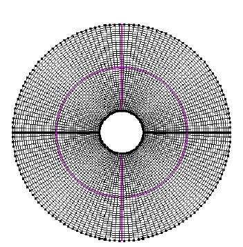

Fig 1.2 The Point Creation tool under the Geometry tab

Enter “0” in the X Value, Y Value and Z Value, next press Preview and Apply. In
this way the point with specified coordinates is created.
Next from the Geometry tab, select Circle creation ->Cpt-Rad Arc (fig. 1.3).

                          Fig. 1.3 The Arc Creation Tools

In the Point creation select the Pick Existing and click with the left mouse
button in the (0,0,0) point, which will be a central point of the created arc.

In the Arc->Cpt-Radius menu enter the following:
Radius: 1
Start Angle: 0
End Angle: 180
Press Preview and than Apply. Fig 1.3 shows results of our work.

               Fig 1.3 Half of the arc created using Arc Creation Tool

In the same way create another arc. Use the central point (0,0,0), and the
following parameters:
Radius: 5
Start Angle: 0
End Angle: 180
The project should look like in fig. 1.4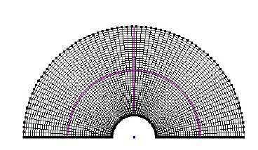

Fig. 1.4 The two concentric arcs

From the Geometry tab, choose Line creation -> Line.
Select the first point of the bigger arc and next, first point of the smaller one and
press the middle mouse button or Apply to create the line. In the same way
create the line between the final points of arcs (fig. 1.5).

                     Fig. 1.5 The basic geometry of the project.

2. Creating Structured face
From the Grid tab, select Structured Edge options -> Create(Edit) structured edge
(fig 2.1):

 Fig 2.1 The Create Structured Edge tool

                                             Fig. 2.2 the Create edge control panel

The Edge -> Create control panel appears (fig. 2.2).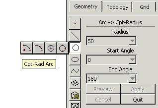

Enter “72” in the Number of Points field,
Select the outer arc and press Apply,
Select the inner arc and press Apply.
In this way we created the edges on the outer and inner arcs.

Next,
Enter “40” in the Number of Points field,
Select the line that connects the left sides of the inner and outer arc and press
Apply,
Select the line that connects the right sides of the inner and outer arc and press
Apply.
In this way we created edges on the lines that connect the arcs.
Using the 4 edges we have to create the structured face.
Select Structured Face Options -> Create Structured Face (fig. 2.3).

                     Fig. 2.3. The Create Structured Edge tool

In the Face-> Create control panel select Edge Sets.
Next, click all the edges and make sure that the middle mouse button was
pressed after each edge selected. Click Apply. The structured face grid appears as
shown in fig. 2.4:

                            Fig. 2.4. The structured grid

3. Rotating the model
Under the Geometry tab, select Rotate -> Rotate Entity (fig. 3.1). Then select the
face handler (see fig. 3.2) and press the middle mouse button.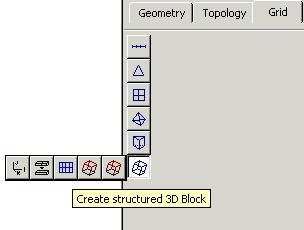

Fig 3.1 The Rotate Entity tool

                                                  Fig 3.2 The Face Handler

From the Rotate -> Entities control panel set the following:
Rotation Mode: 0
Rotation Angle: 180
Repeat (time): 1
Options: Duplicate
Click Apply.
The model should appear as shown in the figure 3.2:

                            Fig. 3.2 The gridding system

4. Creating structured 3D block
Under the Grid tab, select Structured Block options -> Create structured 3D
Block (fig. 4.1).

                    Fig. 4.1 The Create Structured 3D Block tool

In the Block -> Create panel choose Extrusion. Select each of the handlers and
press the middle mouse button. From the Block -> Create control panel set the
following:
Extrude options: Z
Distance: 0.1
Number of Points: 3
Create: Multiple Blocks
Click Apply.

5. Saving the model
Save the model as your_name.GGD file in directory of your choice. This file allows
you to edit this model later in CFD-GEOM. Next, save the model as
your_name.DTF file. This file contains the information about the mesh necessary
to run simulations in CFD-Maxwell.

Part Two
Setting up the electromagnetic simulation parameters
              - CFD Maxwell Processing
6. Opening the CFD-Maxwell
Launch the CFD-Maxwell and open the .dtf file using the menu command File ->
Open. Click the PT (Problem Type) and verify that Maxwell checkbox is marked.

7. Setting up a Model Options (MO)
In the Shared panel, in the Transient Time Step select:
Enter Number of Step = 2000
CFL Number = 0.3388036703
The CFL number is cause the time step size to be dt=5e-11. This value will ensure
numerical stability.

In the Maxwell panel select:
Model: Tome Domain
Formulation: Scattered Wave

8. Setting up the Volume conditions (VC)
Select the VC panel. The parameters connected with the material properties
should be defined in this panel.
Select both entries in lower left window.
Change Properties to Solid under the VC Setting Mode area.
Leave all values on their defaults (εr=1, µr=1, σ = 0 [S/m])
Click Apply.

9. Setting up the Boundary Conditions (BC)
Select the BC panel.

Click on the “front –view” button or choose menu View -> Front.
Select the both half – circular faces by clicking on their center points and keeping
the CTRL key pressed
Select Extrapolation as boundary Sub Type
Click Apply

Turn the model around by pressing the “Back View” button or picking menu View
-> Back.
Select both half – circular faces and select Extrapolation as boundary Sub Type.
Click Apply

Turn the model until you see edge faces (fig. 9.1).

                                      Fig. 9.1

Select the both faces by clicking on their center points and keeping the CTRL key
pressed.
Select Perfect Conductor as boundary Sub Type.
Click Apply.

10. Setting up the Initial Conditions (IC)

Select the IC panel.
Under IC Global Settings choose: For all Volumes
Set the following values:

Electric field Propagation Vector: X=1
                                   Y=0
                                   Z=0
Polarization Vector:               X=0
                                   Y=1
                                   Z=0
Amplitude: 1 V/m

Under the Evaluation Method select: Sinusoidal
Enter 100MHz as frequency.
Click Apply.

11. Setting up Solution Control parameters

Select the SC panel.
Choose the Graphics sub-panel.
Pick all variables (which will be saved to the output file) containing the magnetic
flux density B.

Select the Output sub-panel.
Choose the “Unique Filename”
and Enter 100 as Timestep Frequency.

12. Running the simulation

Before running the simulation, save your file.
Click on the Run panel and click on the Submit button to start the simulation
process.
You can press View Residuals or View Output buttons to see real-time displays of
the residual history and output of the file contents.

Part Three
Visualization of the results of the calculations
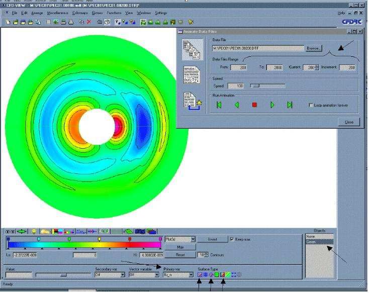
13. Simulation Post Processing in CFD – VIEW
Go to CFD – VIEW window and open the DTF file. In menu File -> Import DTF or
Plot 3D choose your_name.00200.DTF.

In the Objects window in the bottom-right corner of the screen select Geom. From
the toolbar select the following buttons:
Outline: on
Contours: on
Smooth Surface: on

Select the variable you want to display in Primary Variable pull-down menu, e.g.
Bz_n for z component of magnetic flux density.

To view results of many subsequent time steps, saved into separate DTF files
in your current directory, you may use the data-file animation feature in CFD –
VIEW:
– from the menu, select Gizmos – Animate Data File
– in the Animate Data File window, type appropriate values in the Data Files
   Range fields:
   From:        200
   To:          2000
   Current:     200
   Increment: 200
– use Run Animation button to play the sequence of your transient simulation
   results
– you may also use the little up and down arrows nest to Current: step number,
   to step through available DTF files with results

          Fig 13.1 The CFD-VIEW gui with Animate Data Files window.

Part Four
The Project
14.Project
Lets change geometrical model through addition of the second perfectly
electrically conducting (PEC) cylinder (see fig.14.1).

                                             Propagation area

                                                   First
                                                   cylinder

                                             Second cylinder

                          Fig. 14.1 The modified geometry

In the first cylinder the electric field propagation vector, polarization vector and
amplitude of electric field are left unchanged.
In the second cylinder set polarization vectors’ directions as opposite:
   - electric field propagation vector (X=-1, Y=0, Z=0)
   - polarization vector (X=0, Y=-1, Z=0)
or change value of amplitude.

Compare the results with solution obtained in the tutorial. Write down your
conclusions.